2.5. Active Filters
2.5.1. Introduction
In the last two courses we’ve learned about OpAmps and filters. We will be discussing OpAmp filters in this course, which are also known as active filters. We will explore the reasons why OpAmps are used in analog filters and learn how to design them.
2.5.2. The Why
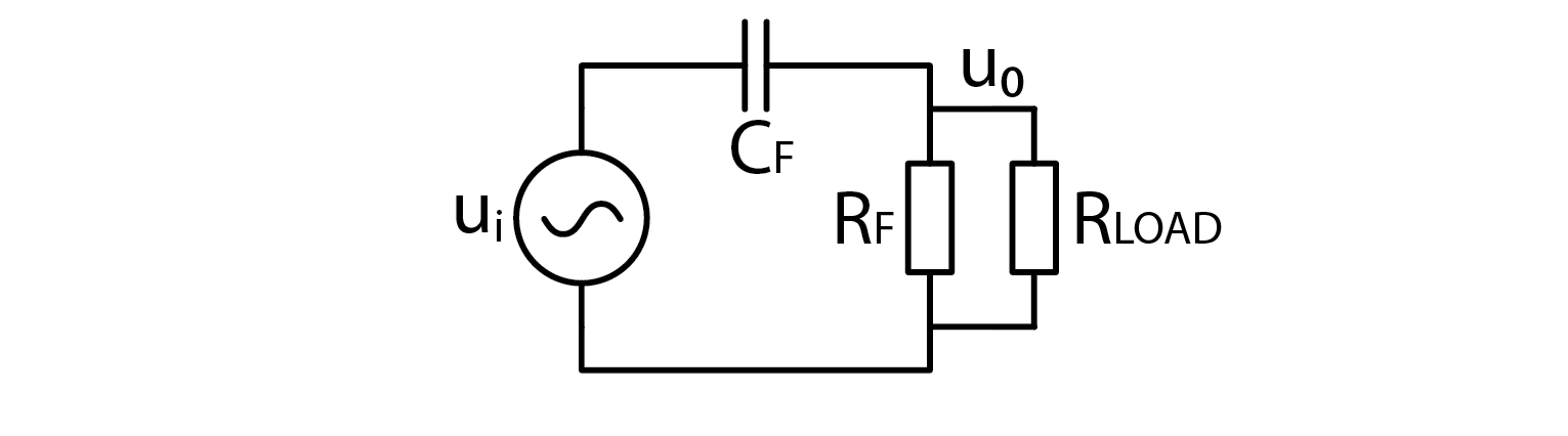
Let us examine the effect of attaching a load to the output of a simple RC high pass filter. Although we know how to compute the filter’s properties in isolation, attaching a resistive load will inevitably modify the filter’s behavior. This is because the newly added load represents an additional resistor in parallel with the filter’s resistor. Whenever two resistors are connected in parallel, they can be combined into a single resistor whose resistance is lower than either of the original resistors, which in turn alters the filter’s cutoff frequency.
Let’s now take a look at a low pass filter, loaded with a resistive load. The two resistors form a voltage divider, meaning that filter will attenuate even DC signals.
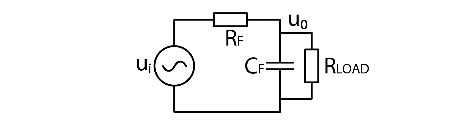
The impact of load on filter performance is more significant when the load impedance is smaller. In contrast, if the load impedance is large, its effect on the filter’s characteristics becomes negligible. It is worth noting that the term “resistance” has been used for simplicity, but the same principle applies to capacitive and inductive loads, although their exact impact may differ from that of resistive loads.
2.5.3. OpAmp characteristics
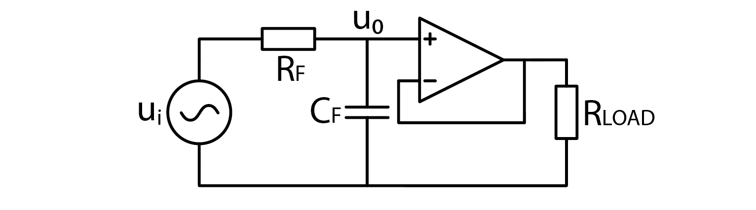
A large input impedance, such as that of an OpAmp, can prevent the load from affecting the characteristics of a filter. By buffering the filter’s output with an OpAmp follower, the load is isolated and the filter’s behavior remains unchanged. To verify this claim, one can perform calculations or simulations. However, there is an even better solution, which will be presented shortly. The following schematic shows the setup for using an OpAmp buffer:
2.5.4. Second order low pass filter
OpAmp followers are great for buffering regular analog filters, but by adding another RC pair, we can create a second-order low pass filter for even better filtering performance. The detailed explanations of how this works can be found in relevant literature, but here is the schematic:
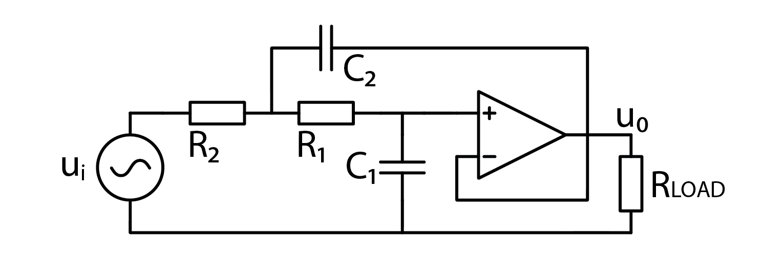
The perceptive readers may observe a familiar RC low pass filter, followed by an OpAmp follower. However, the remaining part is less straightforward. The cutoff frequency of this filter is computed as follows:
\[f_C=\frac{1}{2\pi\sqrt{R_1 C_1 R_2 C_2 }}\]
2.5.5. Second order high pass filter
The schematic for a second order high pass filter is not surprising, as it is the same as the previous circuit for a second order low pass filter, with the positions of resistors and capacitors switched. The corner frequency is also the same. See the schematic below:
2.5.6. Second order filter benefits
Good question! From what I’ve told you so far, second order filters require an OpAmp and extra pair of resistor and capacitor. Let us explore the benefits of second order filters. The first, and the most prominent one, is greater signal attenuation slope. First order filters’ slope is 20 dB/decade. Each additional order adds another 20 dB/decade, meaning that second order filters have 40 dB/decade attenuation slope. And yes, higher order filters exist as well. Higher order filters also induce more phase shifting. You may recall that standard low pass filter will shift the phase by a total of 90°. This effect is multiplied by the order of implemented filter. This means an ideal second order low pass filter will shift phase by 180° in total.
2.5.7. Band pass filter
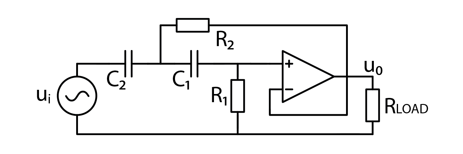
We can construct a bandpass filter using the concept of second order filters. However, it’s not as simple as combining the components from a low pass and high pass filter. In practice, this approach doesn’t work. Instead, we can use an active bandpass filter, which has a different schematic.
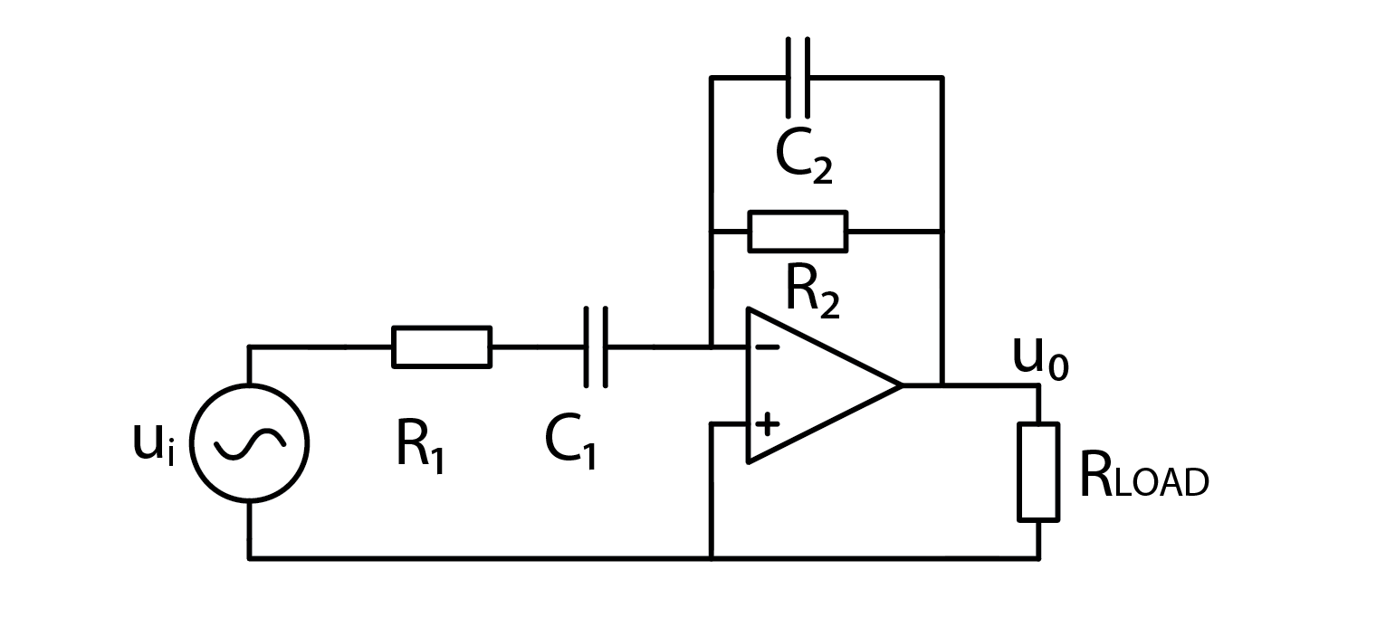
This filter has two corner frequencies. One for high pass and one for low pass portion.
\[f_{HPF}=\frac{1}{2\pi R_1 C_1}\]\[f_{LPF}=\frac{1}{2\pi R_2 C_2}\]
One more special thing about this filter is that it is inverting. Negative gain can also be considered as a phase shift of 180°. It is calculated as:
\[A=-\frac{R_2}{R_1}\]
To avoid diving too deep into the mathematical background, let’s focus on trying out this filter and observing its behavior to gain a practical understanding.
2.5.8. The experiment
Let’s fire up a Red Pitaya and build the circuit.
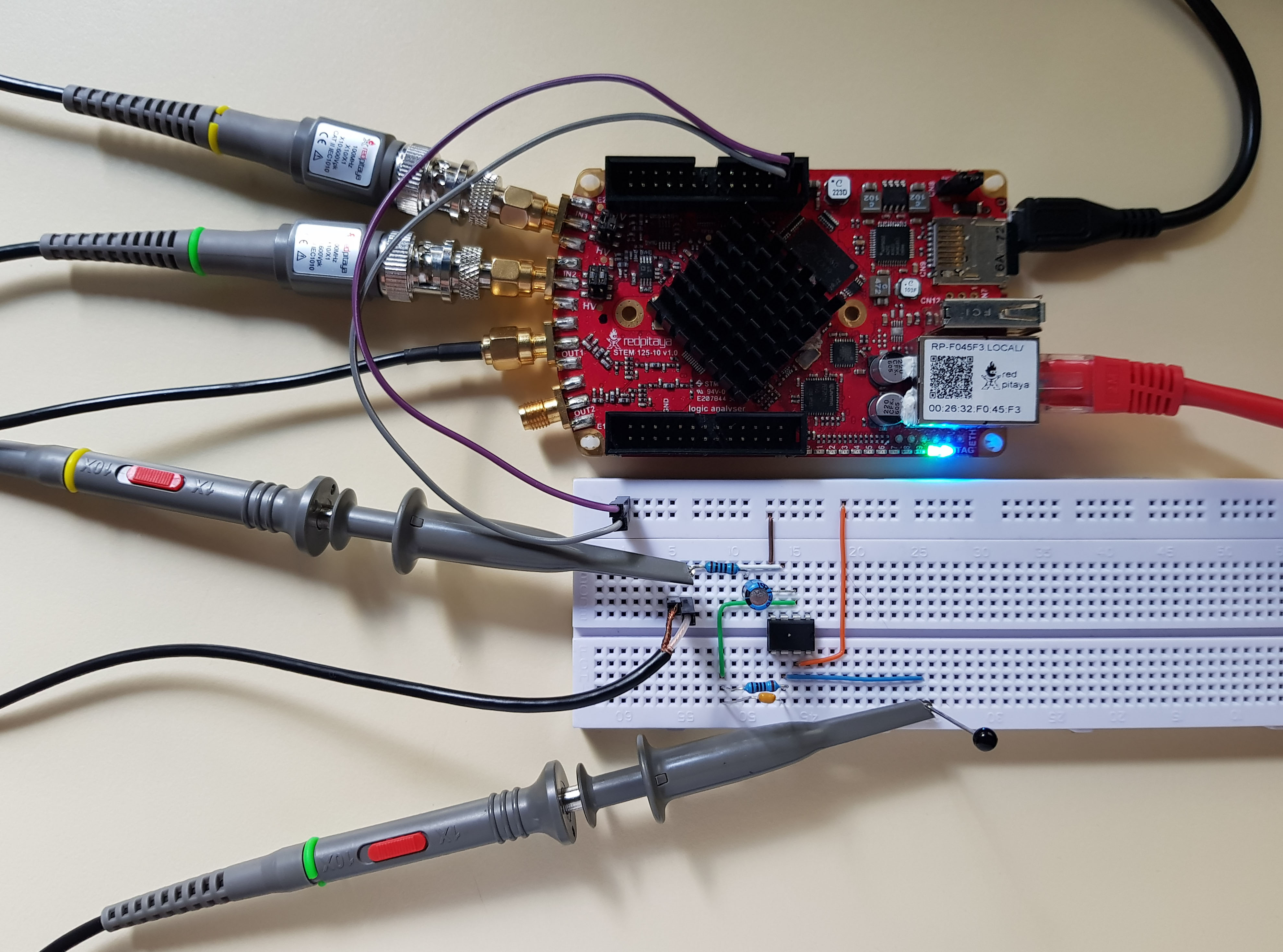
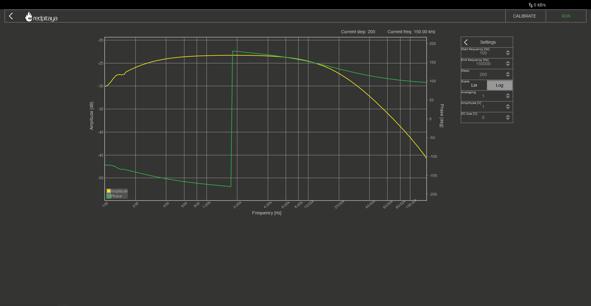
You know the drill. Signal generator channel 1 and input channel 1 to filter input, channel 2 to output. Both probes in x1 mode and run the bode analyzer! Both resistors are 100 ohm, the big capacitor (C1) is 47 uF, the small one is 100 nF, and here is what I got:
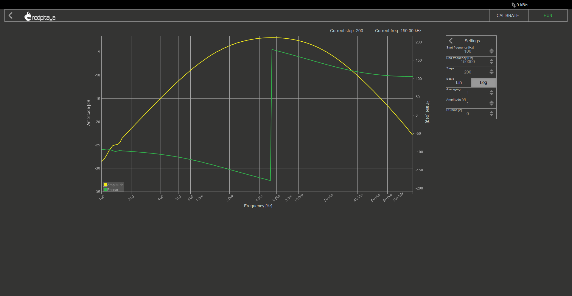
Nothing too special, sure, but we can move cutoff frequencies to alter the filter’s characteristics. This can be done either by changing resistors or changing capacitors. The following bode plot shows filter’s characteristics where C1 or R1 got changed by a factor of 10. I will let the reader try to determine which component got changed. Hint: take a look at the Y axis.
2.5.9. Conclusion
You can play around with the other two active filters we discussed in this course as well but I won’t take any more of your time. Hope you learned something new, if nothing else, that a voltage follower can be used to make sure load doesn’t affect signal shape.
Written by Luka Pogačnik Edited by Andraž Pirc
This teaching material was created by Red Pitaya & Zavod 404 in the scope of the Smart4All innovation project.