2.11. Function Generators

2.11.1. Introduction

Throughout this course, we have utilized Red Pitaya’s function generator to output different types of waveforms. However, we haven’t delved into how it works. The function generator employs a Digital-to-Analog Converter (DAC), which generates a voltage output that corresponds to the type of waveform selected (sine, triangular, square, DC, etc.). Since DACs (and Red Pitayas) can be expensive, it is economically advantageous to explore alternative function generator options for cost-sensitive applications.

2.11.2. Picking up form where we’ve left

This course builds on the previous one, the one about Schmitt triggers. We ended it by building an inverting Schmitt trigger. The circuit looked as such:

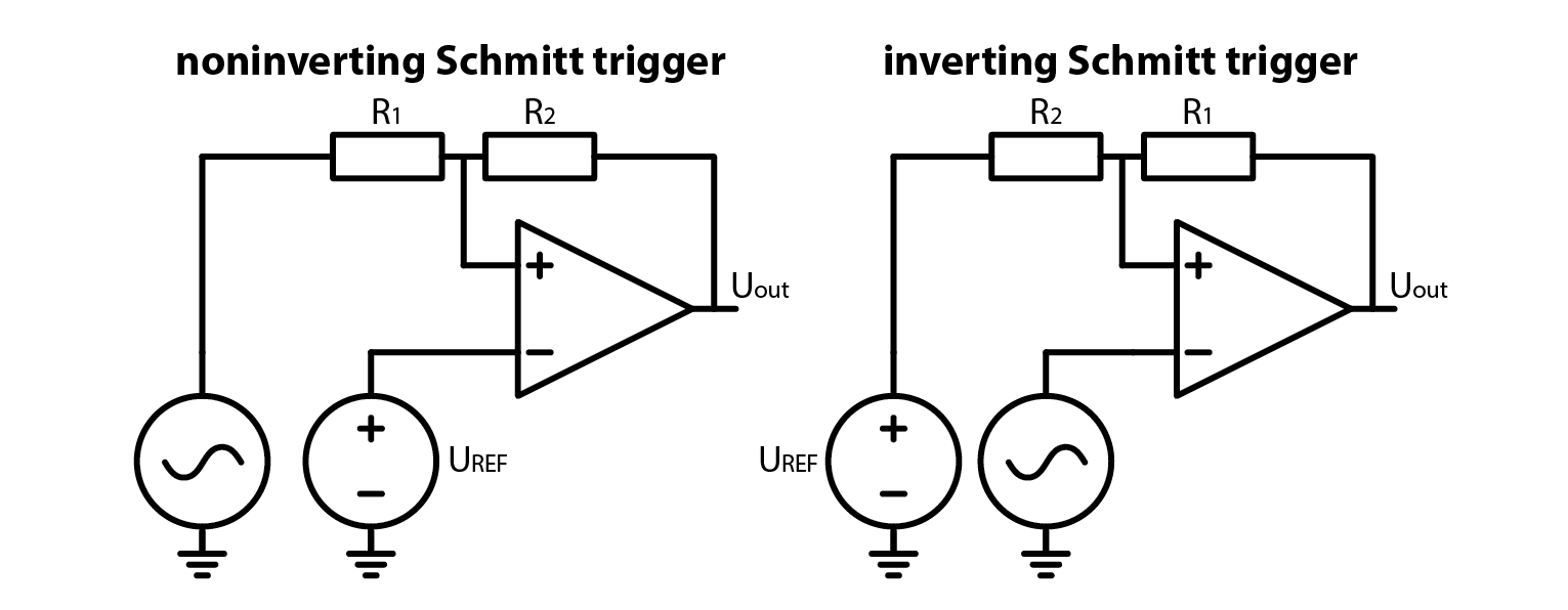
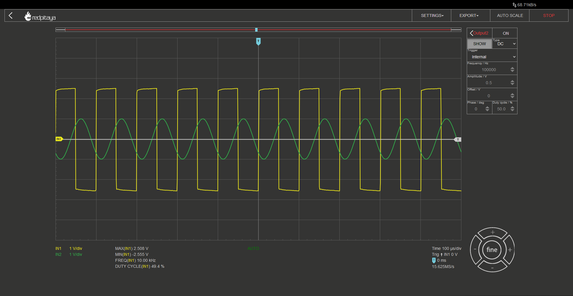
It is worth noting that the OpAmp is supplied from +-3.3 V, as an asymmetric supply voltage won’t work. Let’s make another experiment. What would happen, if we added another resistor to the OpAmp’s output? Answer is the same as the last time. Nothing, unless the resistor was so small that we overloaded the OpAmp’s output. Now here comes the trick question: what would happen if we loaded the OpAmp’s output with an RC low pass filter, a 1 kOhm and 10 nF RC low pass filter, for example? Answer is quite unremarkable. Here is the oscillogram (yellow trace is OpAmp’s output and green one is RC’s middle node):

At first glance, the image of the signal fed through an RC low pass filter may not seem impressive - it resembles a poor quality square wave that takes a long time to settle. However, there is an interesting feature to note: since the circuit is based on an inverting Schmitt trigger, when the input signal exceeds the positive threshold, the output becomes negative, and when it falls below the negative threshold, the output becomes positive. By feeding the filtered signal (the green trace) into the Schmitt trigger, the system can start oscillating!

2.11.3. An OpAmp multivibrator

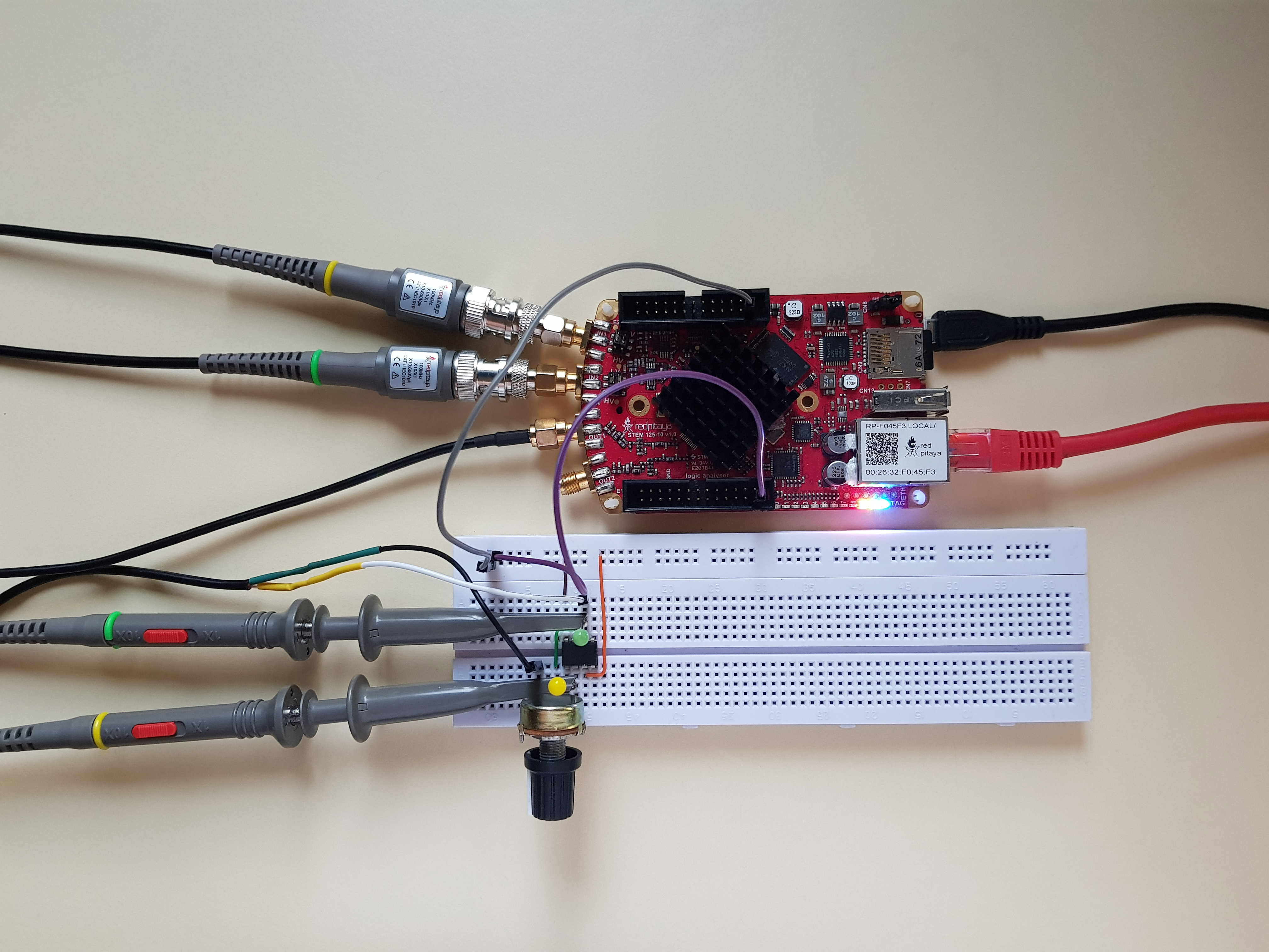
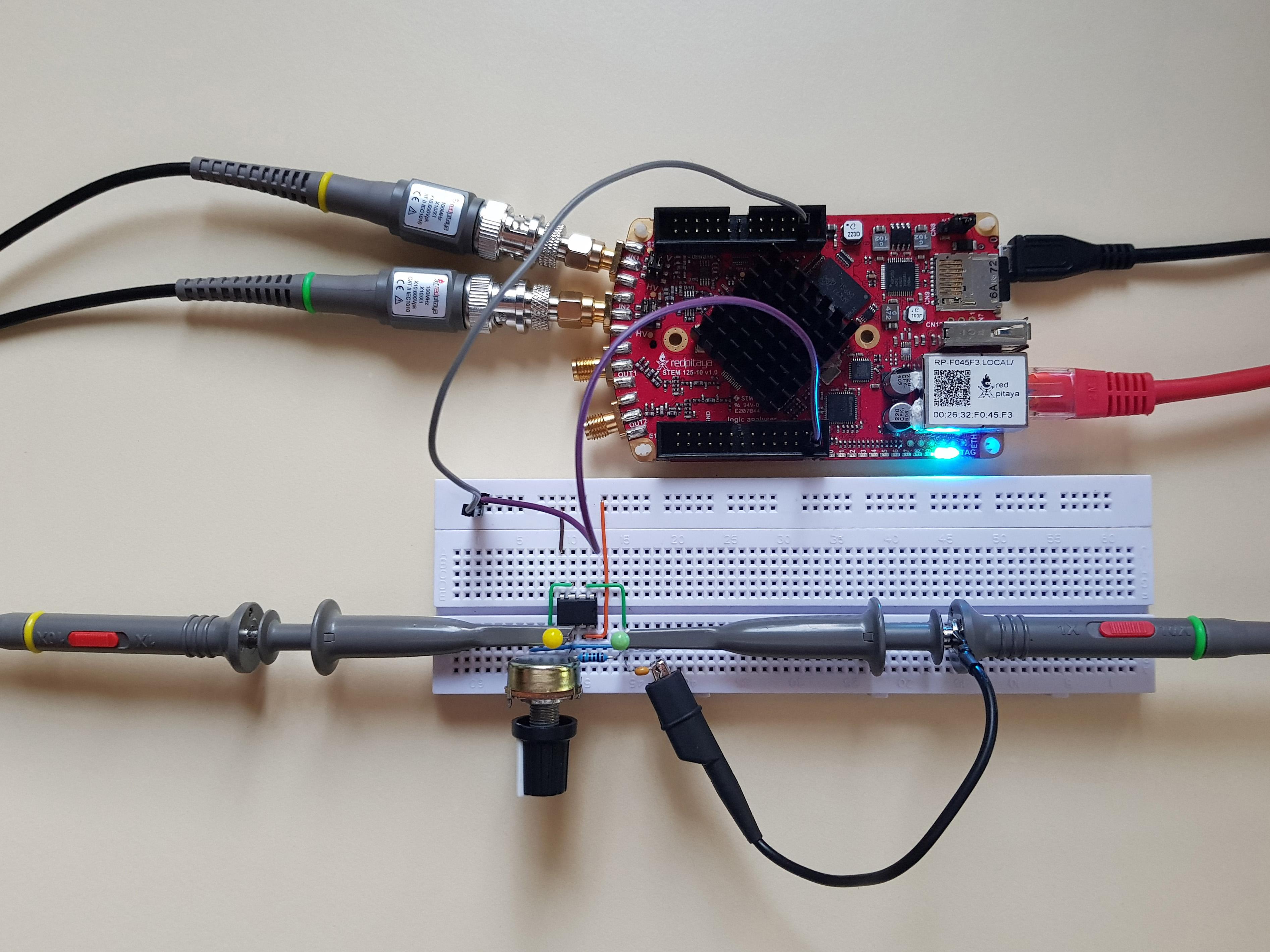
And indeed it does. The circuit we have constructed is formally known as an OpAmp multivibrator. Here are the experimental circuit and the schematic:

You will notice that turning the potentiometer impacts the signal’s frequency. This is due to the changing threshold voltage and thus varying time between output’s transition and RC filtered voltage exceeding the threshold. Here are the equations:

\[\beta = \frac{R_2}{R_1 + R_2}\]

\[T = 2 \cdot R \cdot C \cdot ln(\frac{1+\beta}{1-\beta})\]

\[f = \frac{1}{T}\]

And for those wondering where the \(\beta\) came from, we use it to simplify the equations. We could also use it in equations for the inverting Schmitt trigger:

\[U_{TH}= U_{sat+} \cdot \frac{R_2}{R_1 + R_2} = U_{sat+} \cdot \beta\]

You have now learned how to build a basic adjustable oscillator that produces a square wave output. However, did you know that a sine wave is actually hidden inside the square wave? It may sound surprising, but it’s true!

2.11.4. Discrete Fourier transform

Up until now, we have used two tools from Red Pitaya’s toolbox: the oscilloscope and the Bode analyzer. Today, we will introduce a new tool: the DFT spectrum analyzer. DFT stands for Discrete Fourier Transform, which is used to identify the spectral components present in a signal. But what are spectral components? Any signal can be represented as a sum of an infinite number of sine and cosine functions, each with its own amplitude and frequency. The DFT tells us the factors for each frequency. This is a simplified explanation, but it will suffice for our purposes today. An ideal square wave with a fundamental frequency of F0 and an amplitude of 1 can be approximated as follows:

\[square(f)=\frac{4}{π} \cdot (sin⁡(F0) + \frac{1}{3} sin⁡(3 \cdot F0) + \frac{1}{5} sin⁡(5 \cdot F0) + ...)\]

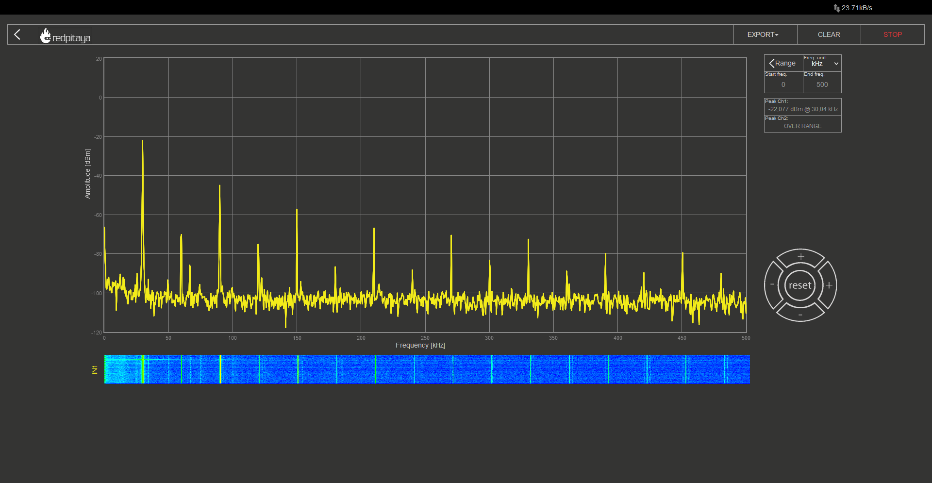
So we would expect our square wave signal to contain the base frequency and its odd multiples. And what do we really get?

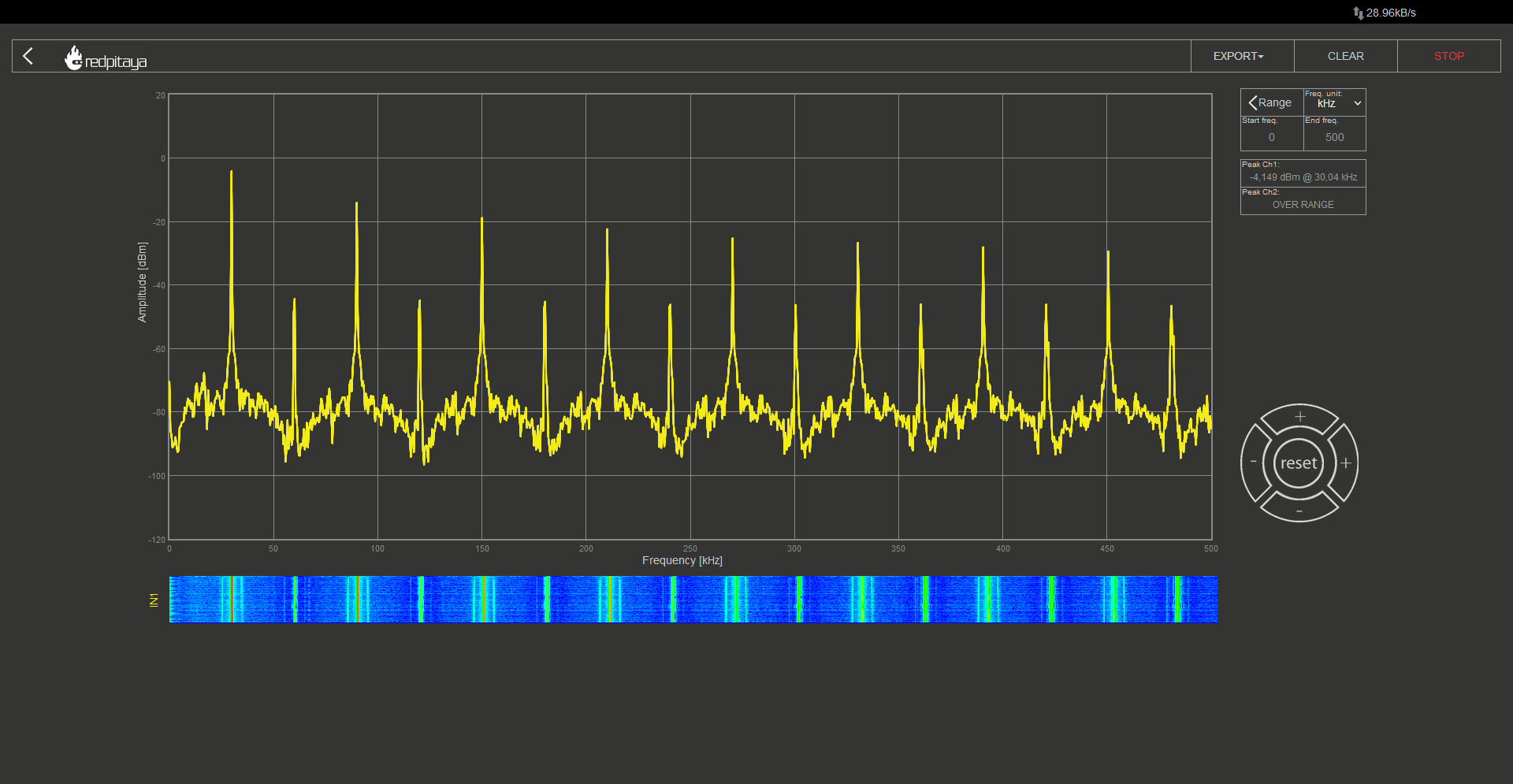
During the experiment, I configured the oscillator to produce a 30 kHz signal and set the DFT analyser to detect frequencies up to 500 kHz. The resulting spectrum showed equally spaced spikes, with odd spikes being much larger than even ones. Keep in mind that the vertical axis is logarithmic. While we anticipated the odd spectral components, the even ones were unexpected. However, we can attribute them to the discrepancy between an ideal square wave and the approximation we generated. Therefore, if we disregard the even components, we can observe the anticipated pattern for a square wave.

Regenerate response

2.11.5. A sine wave generator

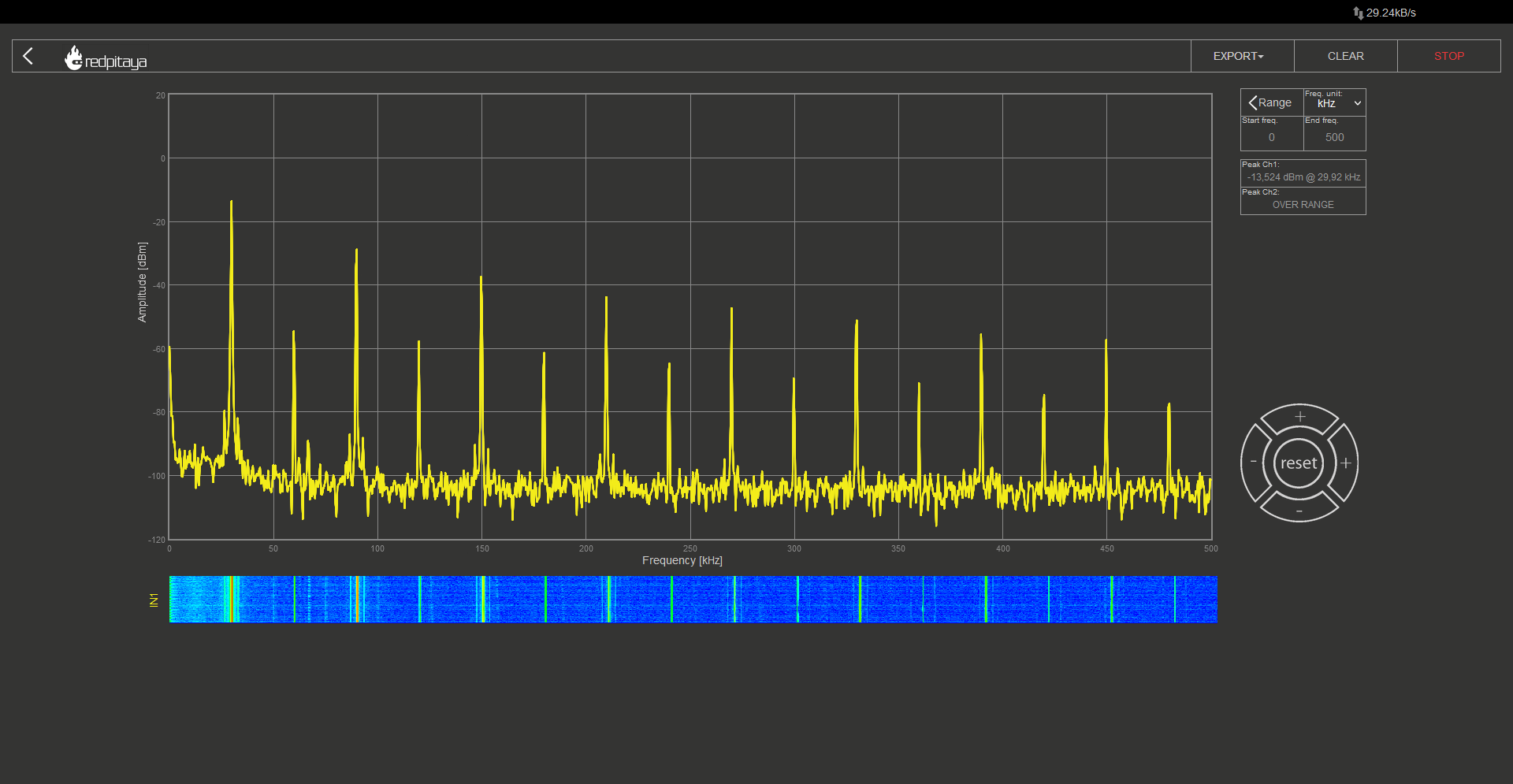
There are dedicated oscillators that produce a sine wave, but as I mentioned before, a sine wave is an integral part of any square wave. We can get to it by removing higher spectral components. We will do it by stringing RC filters one after the other.

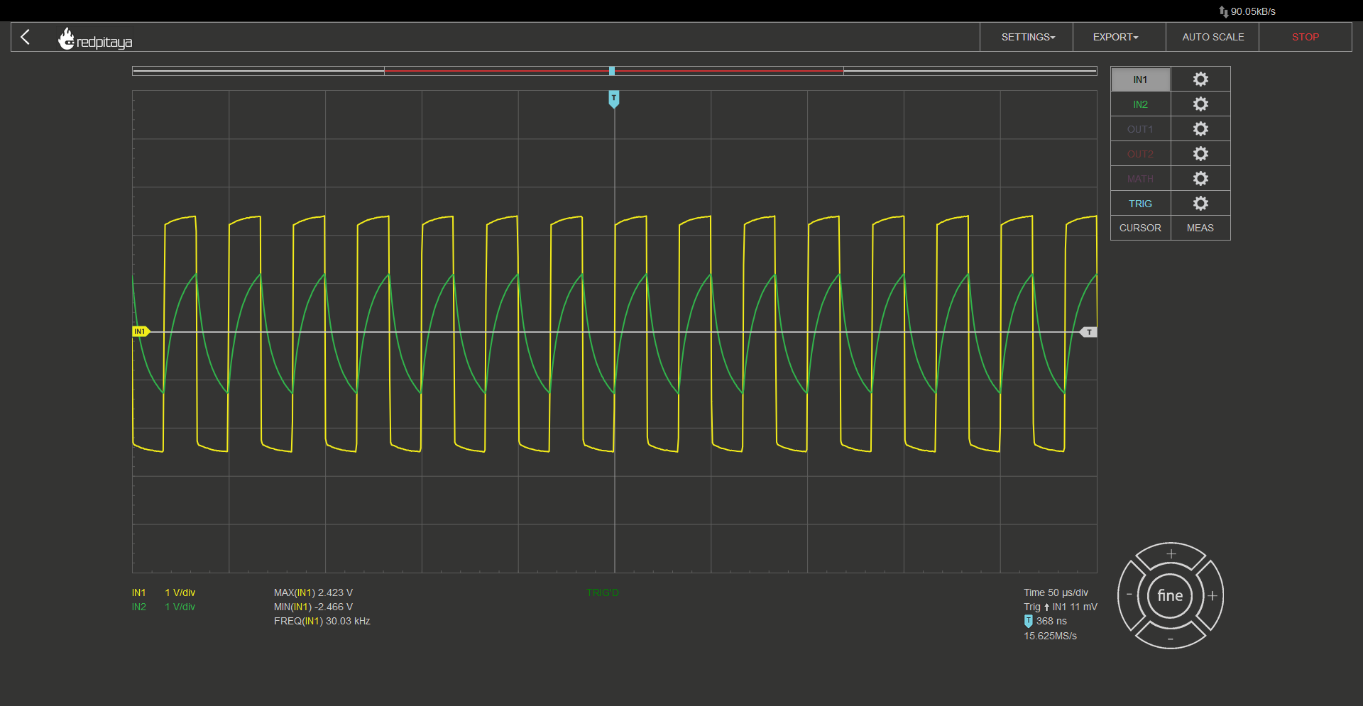
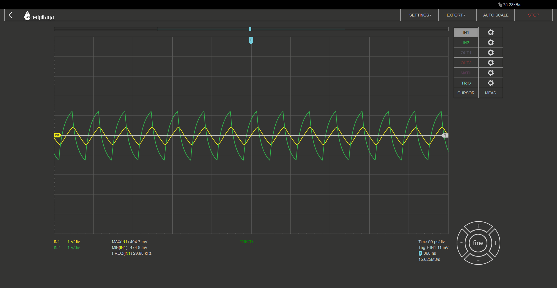
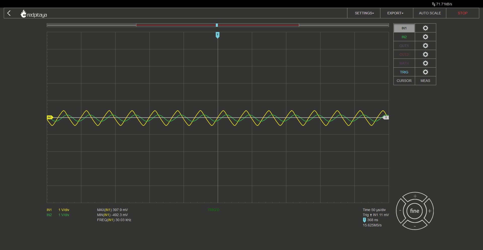
All of the RC filters we will be using a resistance of 1 kOhm and a capacitance of 10 nF, which is the same as the ones we used in our oscillator. It’s worth noting that the corner frequency of such a filter is around 16 kHz, which is approximately half the frequency of the oscillator. This will result in some signal attenuation but will also result in a faster removal of higher spectral components. In the first oscillogram, the yellow trace represents the oscillator’s output, and the green trace represents the filtered output using the same RC filter as in the oscillator. After that, I’m confident you will be able to identify which waveform corresponds to which filter by comparing their shapes.

After first RC:

After second RC:

After third RC:

After going through three stages of filtering, our initial square wave began to resemble a sine wave. However, there are still multiple higher-order components present in the signal’s spectrum. Nonetheless, the fact that the next highest component is attenuated by more than 20 dB in comparison to the first one is significant. A 20 dB attenuation is more than 20 times. It’s important to note that the resulting sine wave is significantly smaller in amplitude than the original square wave. Therefore, an amplifier is necessary to adjust the amplitude. Unfortunately, there is no way around this requirement in this particular oscillator design.

2.11.6. Triangular wave generator

By adding an RC with a time constant that is far greater than the oscillator’s base frequency, we can achieve a proper triangular waveform with sharp corners. Here’s an example of what it looks like:

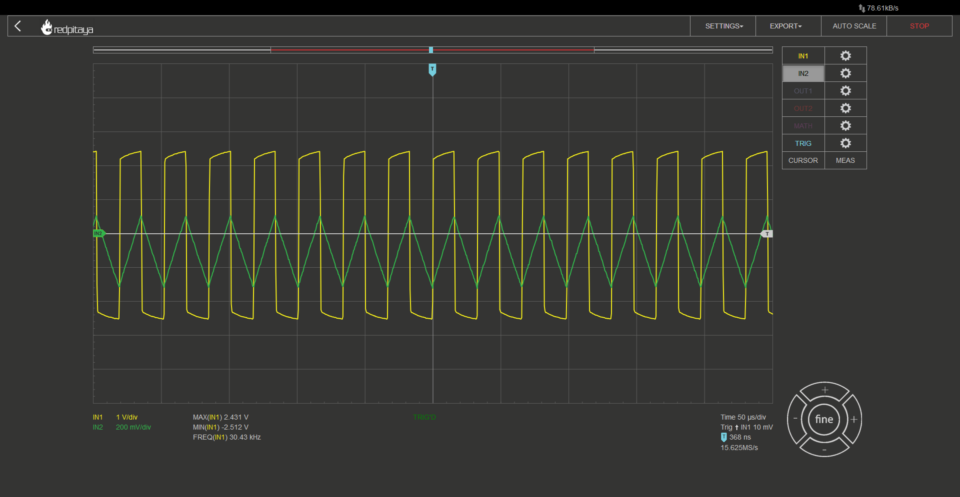
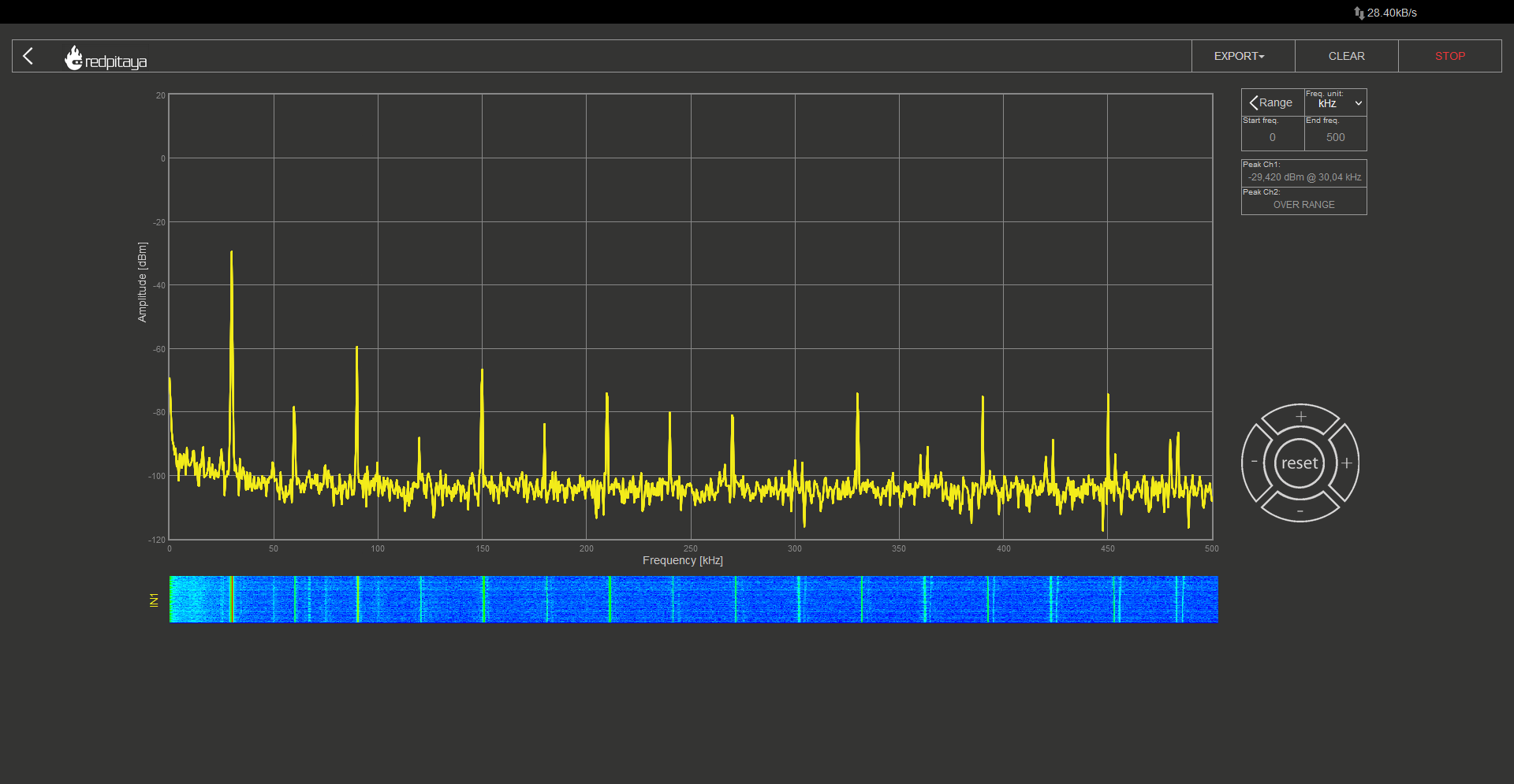
In this example, a 10 kOhm 10 nF RC filter was used to generate a triangular waveform. Although the resulting signal is not technically a pure triangular waveform, it closely resembles one due to the time constant being much greater than the oscillation frequency. To compare it to a true triangular waveform, it is recommended to run it through a DFT and convert the amplitudes of the signal’s peaks from dBm to volts. It is worth noting that the relationship between volts and dBm is proportional, denoted by the symbol \(\propto\)

\[U \propto 10^{P_{dBm/20}}\]

Triangular waveforms consist of base frequency and odd multiples (same as square wave) with amplitudes of those spectral following this equation:

\[a_n = \frac{2 \cdot amplitiude}{n \cdot \pi} sin(\frac{n \cdot \pi}{2}) , n=[1,2,5,...)\]

2.11.7. Conclusion

Throughout this course, we have covered the basics of oscillator design, DFT analysis, and waveform conversion from square waves to sine or triangular waveforms. However, it should be noted that the oscillator design discussed in this course is only one of many designs available. Interested individuals are encouraged to explore the internet to learn about oscillators that naturally produce sine waves or other waveforms, such as sawtooths or asymmetric square waves. In conclusion, we hope you found this course informative, and until next time, we bid you farewell.

Written by Luka Pogačnik Edited by Andraž Pirc

This teaching material was created by Red Pitaya & Zavod 404 in the scope of the Smart4All innovation project.