2.2. Transient Response
2.2.1. Objective
The objective of this activity is to inform reader about transient response on a simple circuit that consists of resistors and either capacitors or inductors.
2.2.2. Background
It is a well-known fact that in DC conditions, capacitors behave as open circuits and inductors act as short circuits. This assumption is typically made assuming that inductors have no series resistance and capacitors have no parallel resistance, which is often a valid approximation. However, when dealing with time-varying signals, such as when a voltage source is suddenly connected or disconnected, this assumption may not hold true.
To elaborate on the above-mentioned concept, capacitors resist changes in voltage, while inductors resist changes in current. This behavior can be quite useful in certain circuits and applications, and it is important to take into account when designing and analyzing circuits that involve capacitors and inductors.
2.2.3. Capacitors
Capacitors exhibit a characteristic behavior in which they resist sudden changes in voltage, but not necessarily changes in voltage overall. When a voltage is applied to a capacitor, the capacitor will charge slowly over time. Similarly, when a capacitor is discharged, the voltage across it will decrease slowly. However, current flow in a capacitor can change rapidly. This behavior can be mathematically described by the equations:
\[u_C = \frac{1}{C} \int i_c \cdot dt\]\[i_C = C \cdot \frac{du_C}{dt}\]

In this scenario, we have an R-C circuit that experiences a step change in input voltage from 0 V to :math: ‘U_0’. We can observe how the capacitor behaves in response to this change.
\[u_C = U_0 (1-e^{-t/\tau})\]\[i_C = \frac{U_0}{R} e^{-t/\tau}\]\[\tau = R \cdot C\]
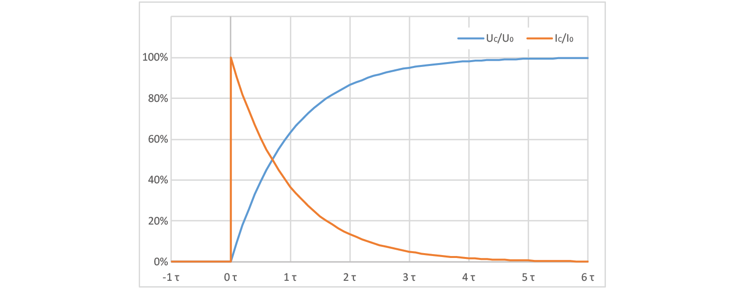
We possess a set of two equations that pertain to voltage and current, respectively, along with a constant denoted by a T-shaped symbol. This symbol is commonly referred to as “tau” and represents the time constant. We will now examine the voltage across a capacitor at various points in time, where time is a multiple of the time constant denoted by the mathematical symbol :math: ‘tau’.
\(t\)
\(U_C / U_{C_{MAX}}\)
\(I_C / I_{C_{MAX}}\)
\(0 \cdot \tau\)
00.00%
100.00%
\(1 \cdot \tau\)
63.21%
36.78%
\(2 \cdot \tau\)
86.46%
13.53%
\(3 \cdot \tau\)
95.02%
04.98%
\(4 \cdot \tau\)
98.16%
01.83%
\(5 \cdot \tau\)
99.32%
00.67%
\(6 \cdot \tau\)
99.75%
00.24%
It can be observed that the voltage across a capacitor reaches over 99% of its steady state value after a time interval of 5 times the time constant (5τ), which is why this point is often considered as the final value. Another noteworthy time value is 3 times the time constant (3τ), as the voltage across the capacitor attains exactly 95% of its final level at this point, rendering it easily discernible on an oscilloscope. It is worth noting that the current across the capacitor follows an inverse curve in comparison to the voltage, meaning that the current values can be calculated by subtracting the voltage value from 100%.
Additionally, it should be noted that if the circuit is a CR circuit rather than an RC circuit, the voltage and current equations will be interchanged. Consequently, the voltage across the capacitor will experience a sudden increase, while the current across the circuit will change gradually.
2.2.4. Inductors
We say that inductors resist current change. This works in the same fashion as capacitors resisting voltage change, meaning that current can never change abruptly. The following two equations describe inductor’s voltage and current:
\[i_L = \frac{1}{L} \int u_L \cdot dt\]\[u_L = L \cdot \frac{di_L}{dt}\]

However, if you are not interested in discussing integrals, and would instead prefer a set of standard procedures or guidelines, then I can assist you with that as well. Let’s explore how an inductor behaves when it is subjected to a sudden change in input. For the purposes of this analysis, consider an R-L circuit where the input voltage abruptly increases from 0 volts to a value represented by :math: ‘U_0’.
\[i_L = \frac{U_0}{R} (1-e^{-t/\tau})\]\[u_L = U_0 \cdot e^{-t/\tau}\]\[\tau = \frac{L}{R}\]
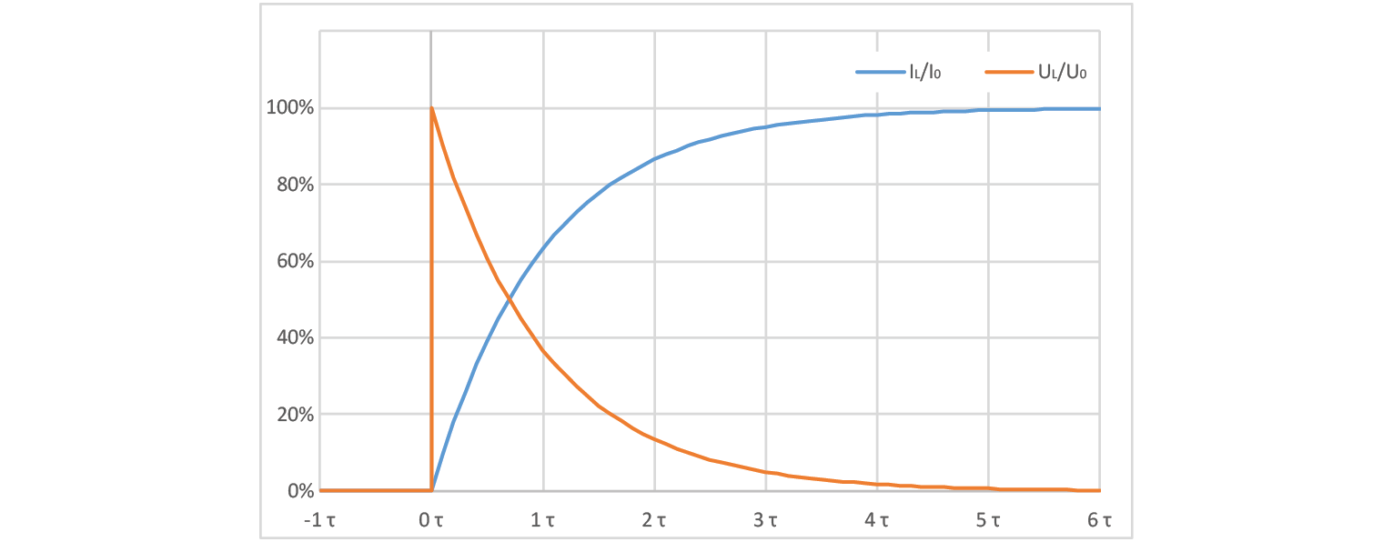
Again we have a set of two equations, one for voltage and one for current and one for the time constant. We can now compare capacitor behavior versus inductor behavior and our theory of inductor having an inverse function of capacitor is confirmed.
\(t\)
\(I_L / I_{L_{MAX}}\)
\(U_L / U_{L_{MAX}}\)
\(0 \cdot \tau\)
00.00%
100.00%
\(1 \cdot \tau\)
63.21%
36.78%
\(2 \cdot \tau\)
86.46%
13.53%
\(3 \cdot \tau\)
95.02%
04.98%
\(4 \cdot \tau\)
98.16%
01.83%
\(5 \cdot \tau\)
99.32%
00.67%
\(6 \cdot \tau\)
99.75%
00.24%
Upon reflection, it appears that the information previously shared regarding capacitors and their behavior has been inadvertently repeated for inductors, with the roles of voltage and current reversed. However, it should be noted that the calculation for time constant (:math: ‘tau’) has been altered. In general, ideal capacitors and inductors are reciprocally analogous, such that only four formulas need to be committed to memory: two for computing the time constant (:math: ‘tau’), one for a rising signal, and one for a falling signal.
2.2.5. What? Please explain…
Let’s take a look at an example. RC circuit, input voltage drops from 5 V to 3 V ( \(U_0\) =-2 V). Since we are looking at capacitor’s voltage, we should expect that it will slowly drop to that value, meaning that we need to find an equation that will equal 0 at t=0. \(e^{-t/\tau}\) fits the bill. Final voltage will therefore be starting voltage + voltage change (3 V in this case). Voltage will follow the following curve:
\[u_C = U_{START} + U_0 (1-e^{-t/\tau})\]\[u_C = 5V - 2V \cdot (1-e^{-t/\tau})\]
However, it is advisable to verify this assertion through experimentation, and a red pitaya can serve as a suitable platform for such testing. It is important to note that the voltage range for this setup is restricted to a maximum of ±1 V. With regard to this topic we can move on to our experiment…
2.2.6. The experiment
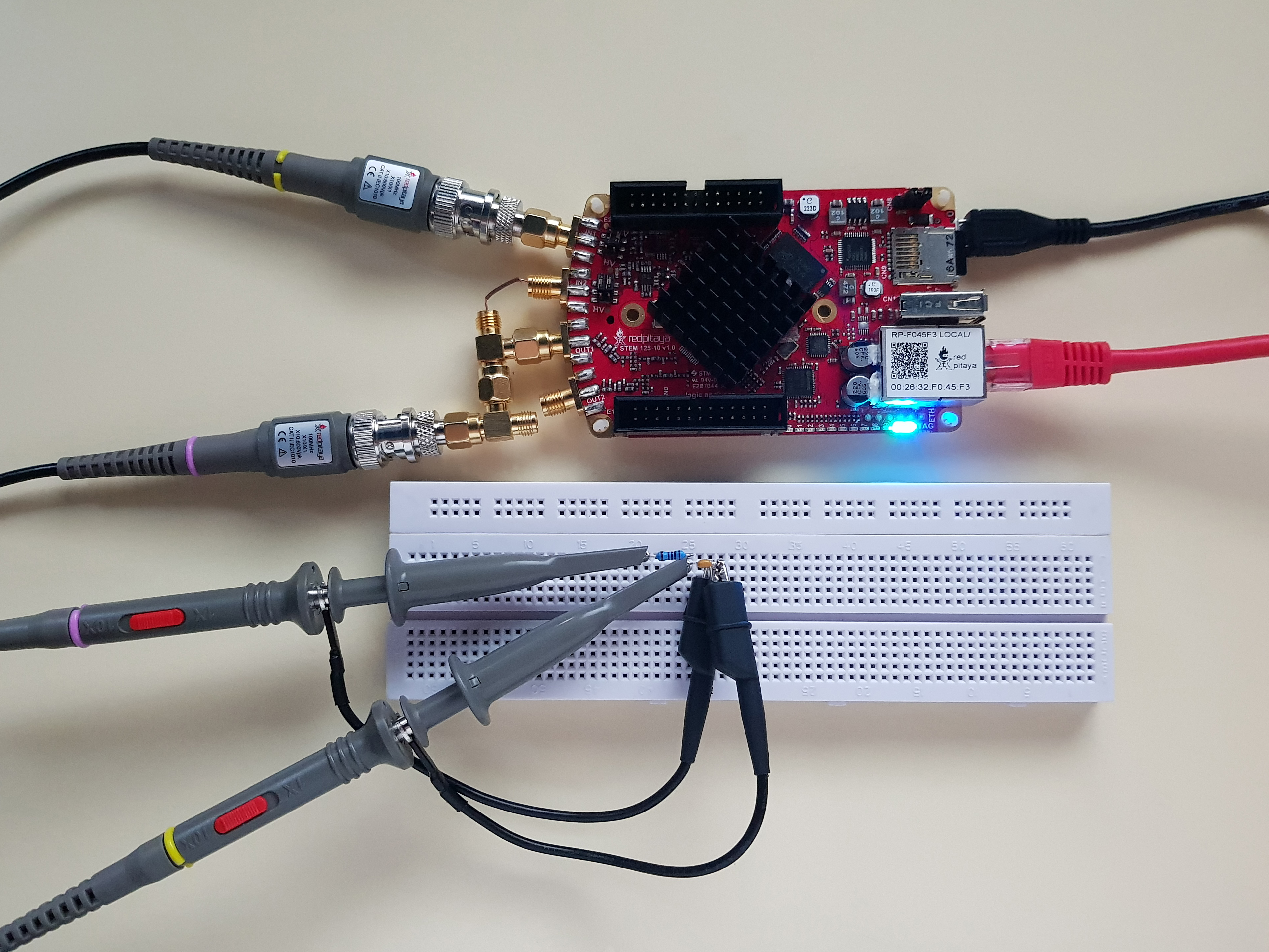
To observe the behavior of a simple RC circuit, it is necessary to connect the probes as follows: Input 1 must be connected to the intermediate node, while the output probe should be connected to the second lead of the resistor. The other lead of the capacitor should be grounded by connecting it to one of the alligator clips. The second input channel should be linked to the Red Pitaya’s output. In the video, a Y splitter provided in the Red Pitaya’s accessories kit was employed, and a wire was utilized to connect the input and output. Although this method may appear rudimentary, it is the simplest way to accurately observe the output signal. Attempting to measure the signal at the same node as the output probe would be impractical because the probes, which are likely to be employed, contain a 100 Ω internal resistance, even in x1 mode, which acts as a part of a voltage divider. It is worth noting that the second Y splitter was added for the sake of tidiness in the accompanying photograph.
With everything hooked up, you have set input 1 to x10 mode (but input 2 in x1 mode, since it’s just a piece of wire with no attenuation), and set Red Pitaya’s signal generator to output a square wave at an appropriate frequency. Appropriate in this case means that it is greater than 1/5τ. I used a 100 Ω resistor and a 10 nF capacitor. Keeping in mind that output probe adds an extra 100 Ω, we get:
\[f_{max}=\frac{1}{10 \cdot 200\Omega \cdot 10nF}=50kHz\]
This will ensure that we can easily observe transient effect without the need to worry about previous transient.
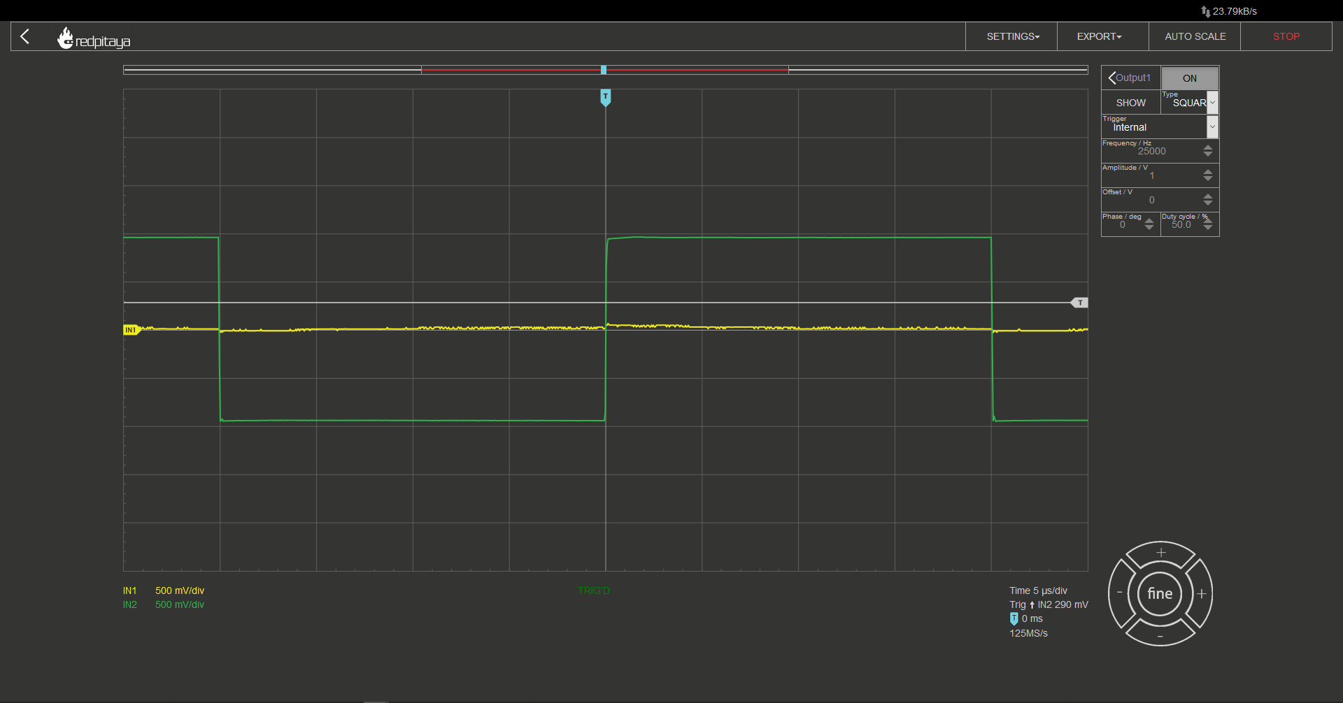
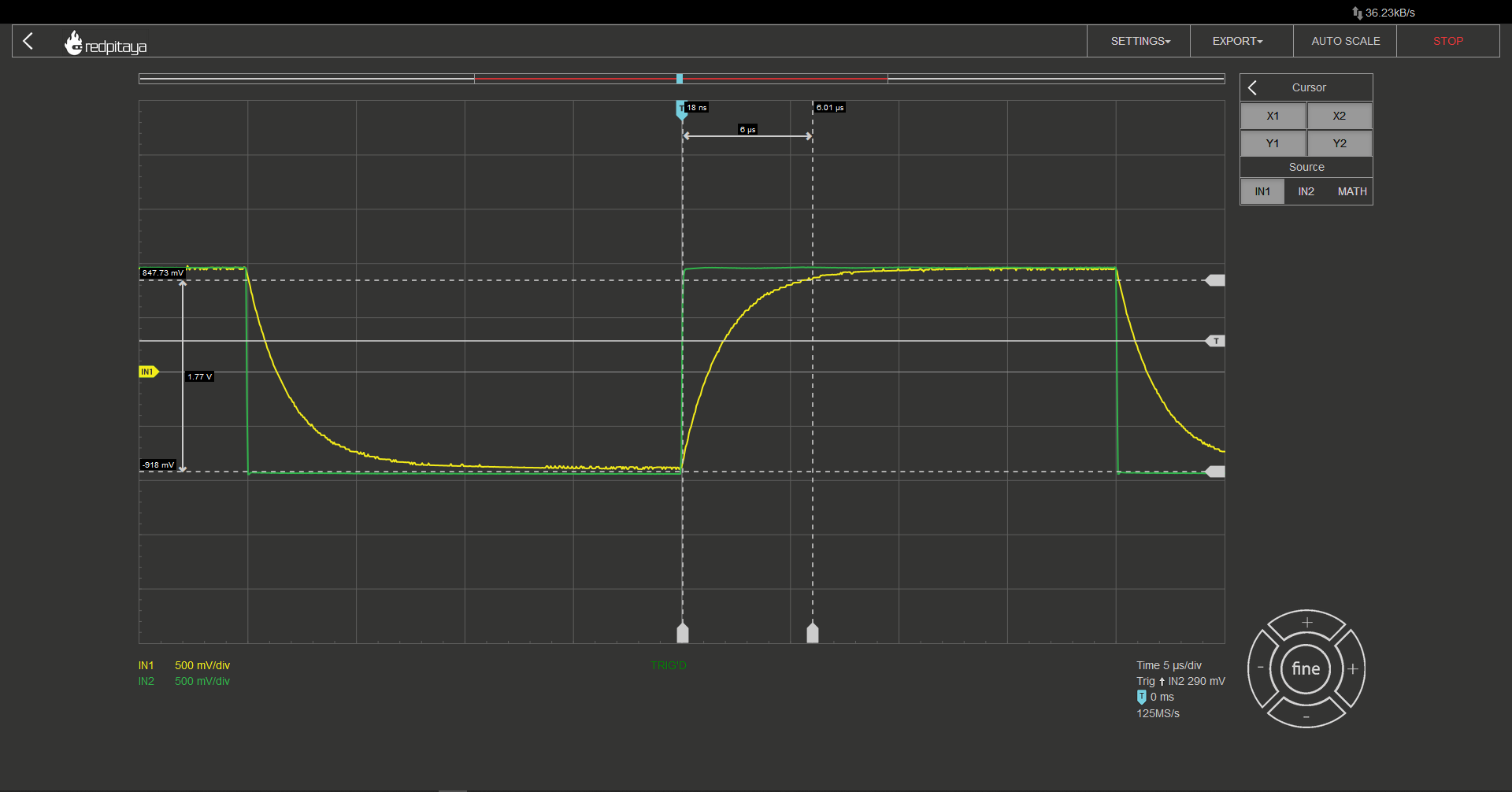
Using cursors, we can measure time for the signal to reach 95% of its change. Since τ = 2 μs we are expecting this measurement to be 6 μs (3τ). Unsurprisingly that is the case. A quick side note: in my case actual peak to peak voltage was 1.85 V, that is why I am measuring time from the start of input change to delta of 1.77 V.
Let’s quickly swap out the capacitor for an inductor. And take a look at the resulting oscillogram.
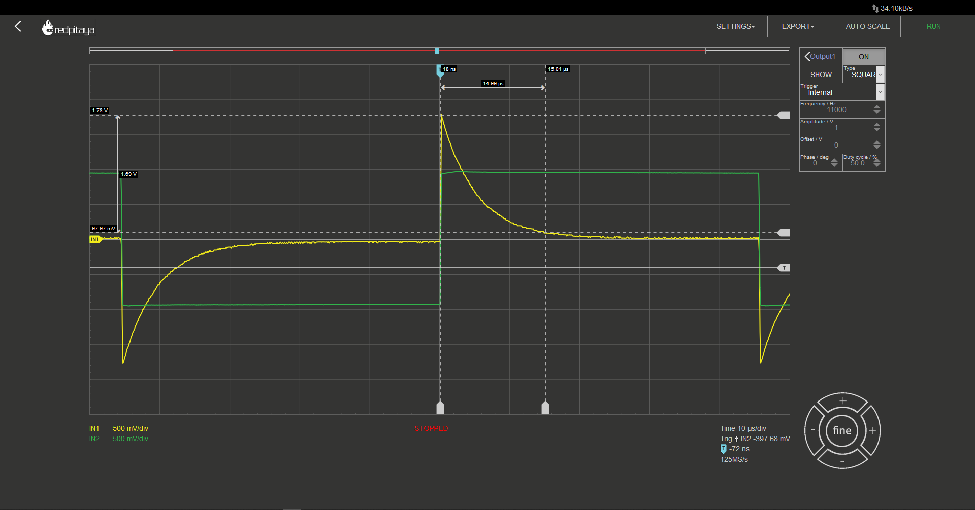
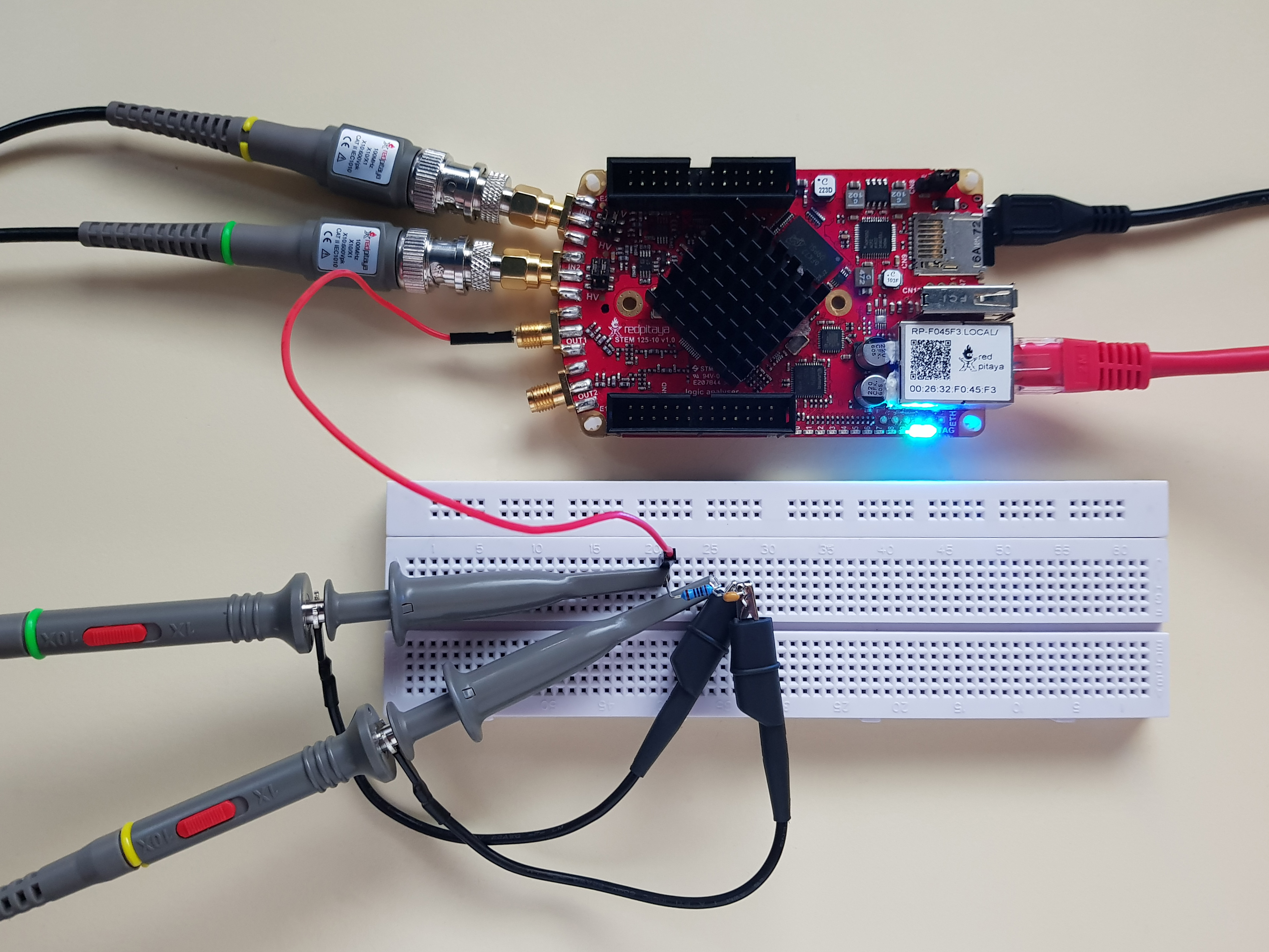
Here we are measuring the time for voltage to move to within 5% of its final value. 15 μs this time. This is because the inductor I used was, 1 mH and the resulting time constant 5 μs. I encourage you to try making RC and CR circuits but be warned; you will have to use something different than an oscilloscope probe to connect signal generator to the circuit or you will have to deal with resistor divider effect, which will reduce steady state voltage. Here is a photo of a “home lab” setup for such measurement. If you have a proper cable, I encourage you to use it instead. Or just mind the voltage divider and use a standard oscilloscope probe. Not that depicted method is a bit flimsy as cables don’t make the best contact with the signal generator. You might want to press on it.
If you make the experiment, you will notice that CR circuit’s oscillogram takes the shape of RL’s and vice versa. I won’t go into detail about why that is, but I will leave you a hint that it has something to do with capacitors and inductors following their respective current curves, current flowing through resistor and you measuring voltage on same resistors.
2.2.7. One last thing
In the video, a question was posed regarding the outcome of conducting similar experiments on an LC circuit. To answer this query, it is recommended to reduce the frequency of the signal generator and perform the experiment. When conducting this experiment, utilizing a low impedance cable to connect the signal generator to the output would be more effective than using an oscilloscope probe.
It is important to note that the results of this experiment will not be revealed at this time. However, it is possible that the outcome may be useful in a future article.
Written by Luka Pogačnik Editted by Andraž Pirc This teaching material was created by Red Pitaya & Zavod 404 in the scope of the Smart4All innovation project.