2.3. Analog Filters
2.3.1. Objective
The objective of this activity is to introduce the reader to the world of passive filter circuits. We will be looking at low-pass and high-pass filters.
2.3.2. Background
In the previous course, we examined the transient response of simple RC and RL circuits. It was observed that a square wave signal is attenuated when passed through an RC circuit. To ensure this effect, we chose an input signal frequency that had a period longer than the settling time of the RC circuit (5τ). Higher frequencies introduce new complexities such as Fourier analysis. For the purpose of this write-up, we will agree that a square wave signal is comprised of a sine wave at the main frequency and an infinite number of sine waves at odd multiples of the main frequency (3, 5, 7…). An RC filter attenuates these components differently based on their frequency, with higher frequencies experiencing greater attenuation. As a result, the signal’s slope is gentler, as observed in the previous course. RC and CR circuits are called filters since they allow some frequencies to pass through while blocking others. It should be noted that this explanation is a simplification, and we will not discuss LR circuits. RL circuits behave similarly to CR circuits, while LR circuits behave similarly to RC circuits. It is also important to note that when discussing signals and frequencies, we are referring to sine wave signals at a particular frequency.
2.3.3. Decibels
Decibels, marked with dB, are a logarithmic unit, used for measuring relative power. To calculate attenuation (or gain) in dB, the following equation is used:
\[G_{dB}=10 \cdot log_{10}(P/P_0)\]
If that wasn’t confusing enough, it should be noted that decibels are typically used to compare power, but we will be using them to compare voltages. This is possible because we know that power is proportional to the square of the voltage, and since exponents inside a logarithm translate to multiplication outside of the logarithm, we can use the following equation:
\[G_{dB}=20 \cdot log_{10}(U/U_0)\]
Simply put, for every 6 dB, the signal is multiplied (or attenuated) by a factor of two. For example, 30 dB corresponds to \(2^5\).
2.3.4. Phase
You likely know what happens if we add a fixed value to a sign function: it shifts left/right by a corresponding amount. This shift is known as phase (\(\varphi\)).
\[f(t) = A \cdot sin(2 \pi \cdot f \cdot t + \varphi)\]
If \(\varphi\) equals \(\pi/2\), the sine function transforms into a cosine function. If the offset value equals \(2\pi\) or a whole multiple of that, the function is seemingly unaltered.
2.3.5. Impedance
Impedance can be thought of as “complex resistance”. It consists of resistance and reactance.
\[Z=R+jX\]
X represents components reactance, which is in a complex domain. It is calculated differently for capacitors and inductors:
\[X_C=\frac{1}{2\pi \cdot f \cdot C}\]\[X_L=2\pi \cdot f \cdot L\]
The j symbol represents complex operator i because in electronics, the lowercase letter i is already reserved for time variable current. Impedance can also be expressed in polar notation as it helps to illustrate the attenuation and phase shifting of the signal.
\[Z=|Z| \cdot e^{j \cdot \varphi}\]\[|Z|=\sqrt{R^2+X^2}\]
Multiplying a signal by \(e^{j \cdot \varphi}\) only shifts its phase by \(\varphi\) without affecting absolute value. This means we can use \(|Z|\) to calculate signal attenuation and \(\varphi\) for signal shifting.
2.3.6. Background math / complex voltage divider
Aside from the name, there is nothing too complex in the underlying math. Voltage divider, where instead of resistances, we are using impedances.

We can recall that output voltage is caluclated as:
\[u_0=u_i \cdot \frac{Z_2}{Z_1+Z_2}\]
When considering only signal attenuation, absolute impedance can be used without complex numbers. This method is similar to calculating resistive voltage divider and only applies to a single frequency, as frequency is necessary for reactance calculation. However, this method does not account for phase shift.
When accounting for different frequencies and phase shifts, complex numbers must be used for calculation. Division by complex numbers may be intimidating, but it is necessary for accurate calculations. An example will not be provided for brevity, as this level of calculation is unlikely to be encountered outside of exams.
With the background information covered, the main topic of the course can be discussed.
2.3.7. Filters
All filters have in common the corner frequency. It is also known as a cutoff frequency. This is a frequency at which the signal drops by 3 dB, which equals 71% of its initial amplitude (\(1/ \sqrt{2}\)). This frequency is calculated as:
\[f_c = \frac{1}{2\pi \cdot R \cdot C}\]
The RC part in the equations presented earlier is denoted by τ, which can be useful in analyzing RL filters.
In simple terms, a low pass filter allows signals below the filter’s corner frequency to pass through with no attenuation and attenuates signals above this frequency at a rate of 20 dB/decade. A decade refers to a range in which the value changes by a factor of ten, such as 1, 10, 100, or 3, 30, or 300.
Regarding phase, it begins to shift one decade before the corner frequency and stops moving one decade after it, resulting in a total shift of 90°. The phase crosses the 45° point at the corner frequency.
In reality, signals seldom behave precisely as described above due to various factors. However, engineers use these simplifications as a starting point until the experimental stage of the analysis.
2.3.8. Low pass filter
As mentioned before, a low pas filter is just an RC circuit.

Let’s construct a low pass filter from a 1000 Ω resistor and a 10 nF capacitor. The calculated corner frequency is 15.9 kHz, idealized graph should look a little like this (not that X axis is logarithmic):
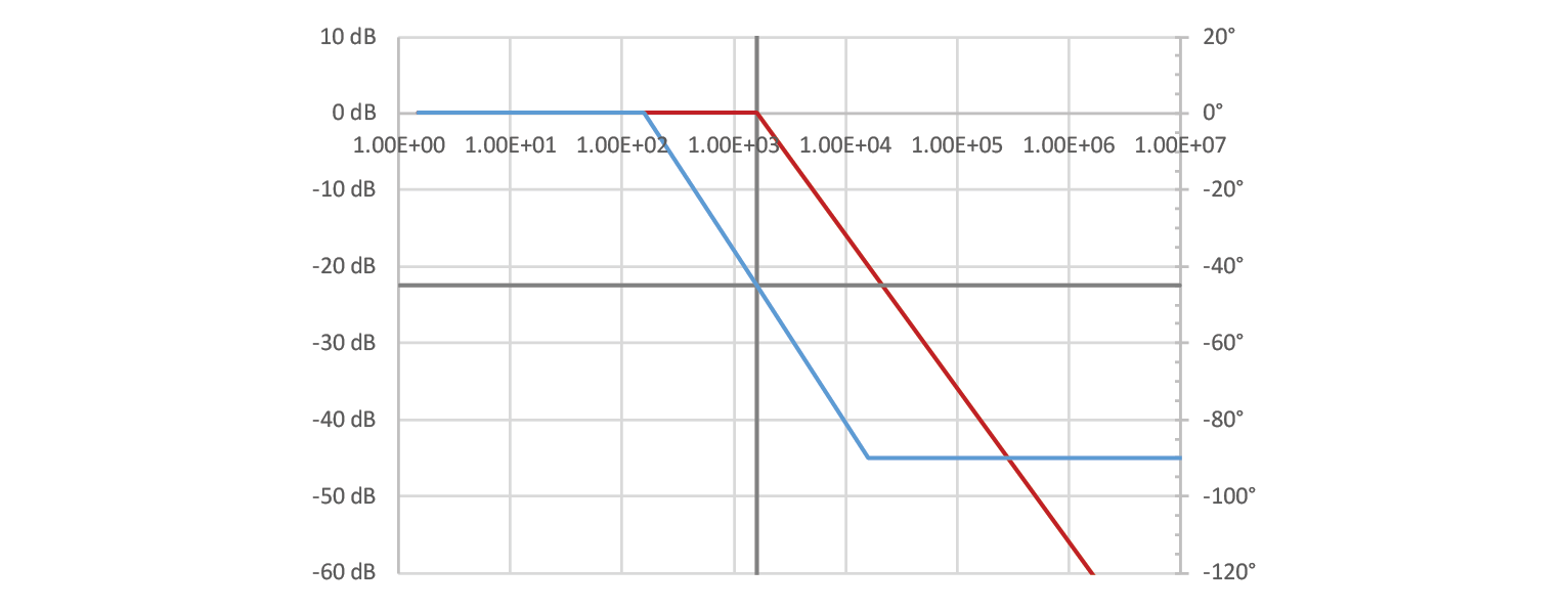
In the simplified representation of low pass filters, signal attenuation is presumed to be absent below the corner frequency, while the phase begins to deviate one decade before and stabilizes one decade after this frequency. It is important to note that this representation conflicts with the commonly used definition of corner frequency as the point at which signal amplitude crosses the -3 dB threshold, as in this simplified representation, attenuation at the corner frequency is zero. This discrepancy can be regarded as a minor detail of little practical significance.
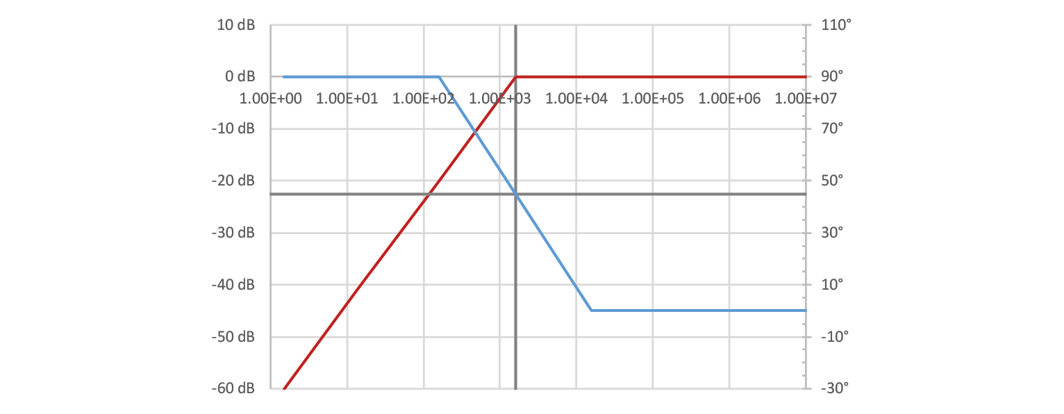
2.3.9. High pass filter
If low pass is just an RC circuit, high pass filter will probably be a CR circuit.
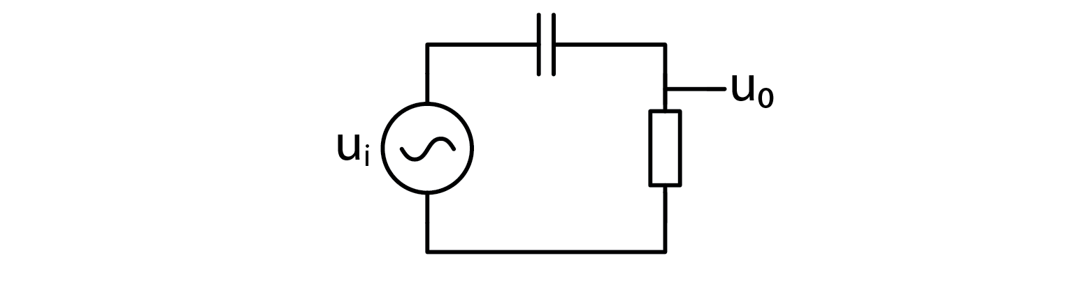
Let’s take a look at the characteristics of such filter, constructed from same components as before – a 1000 Ω resistor and a 10 nF capacitor. Corner frequency will be the same, 15.9 kHz, but the characteristic curves will be different. Note that the phase axis has been altered.
2.3.10. Bode analysis
The process of measuring the characteristics of a filter in a real-world scenario may raise curiosity. The answer to this question is straightforward: we can excite the circuit with a synthesized sine wave at various frequencies within the desired range and then measure the amplitude gain (or attenuation) and phase shift. Red Pitaya offers a built-in bode analysis functionality, which can aid in this process. To better understand this concept, let us construct a low pass filter and connect it to the Red Pitaya device to observe its behavior.
2.3.11. Hands on experiment
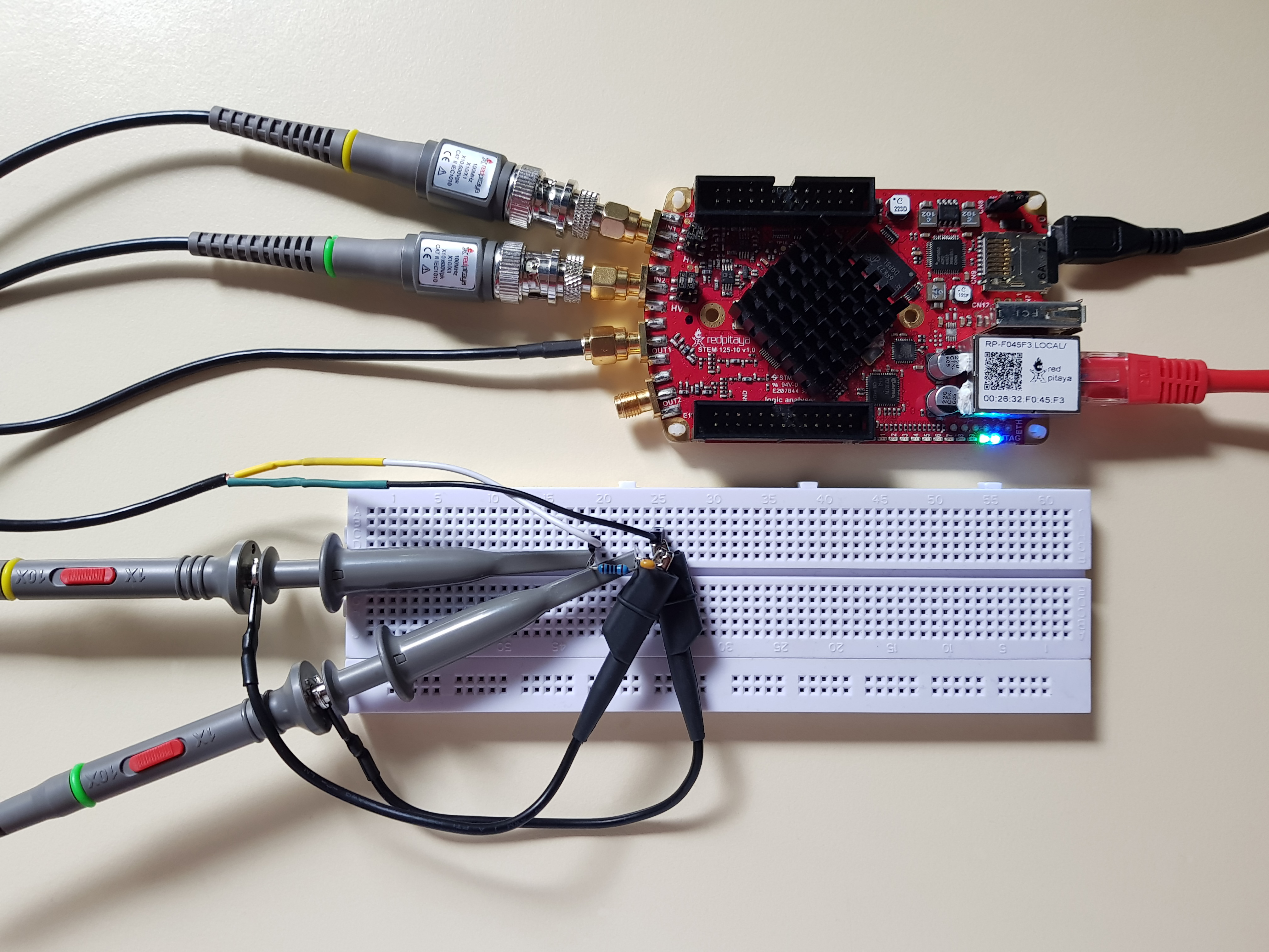
Wiring is important here. If you are ever unsure how to do it, you can always hit “calibrate” button in Red Pitaya’s bode analyzer. Or you can reference this image, that has been taken from RP’s calibration instructions:
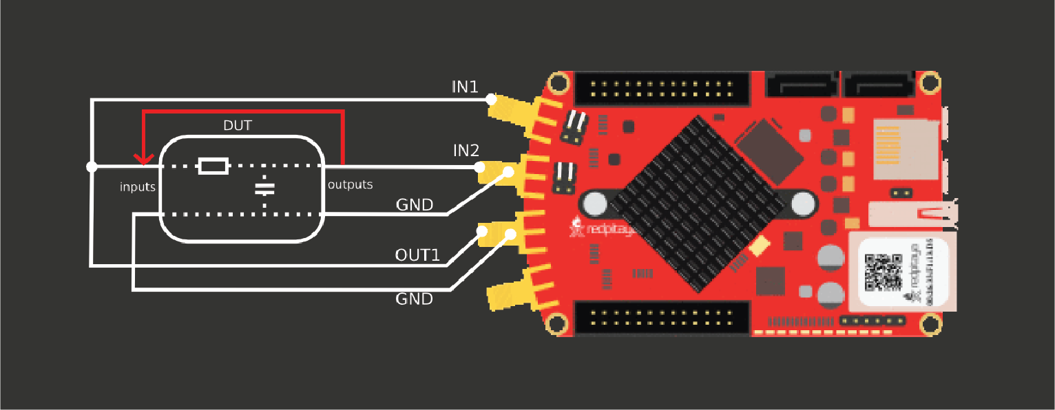
It is important to note that the image does not explicitly state that the probes used in this setup must be in x1 mode and the signal output must have the lowest possible resistance. Using oscilloscope probes in place of a cable is not recommended for this purpose. To ensure proper calibration, the “calibrate” button on Red Pitaya’s bode analyzer can be used as a fail-safe measure.
With that set, connect to Red Pitaya, click Bode Analyser app and bode plot should start automatically. You can stop it as the default settings are somewhat useless. In settings, set appropriate start and stop frequencies and hit Run. I recommend measuring in at least 100 steps. Once measurement completes, you are left with two curves. Yellow one is for gain, and the green one for phase. Note that gain uses vertical scale on the left, while phase’s vertical axis is on the right. If you want to make measurements, you can add cursors. F cursors will snap to frequency, G to gain, and P to phase. Below is a measurement for a low pass filter, using same components as before:
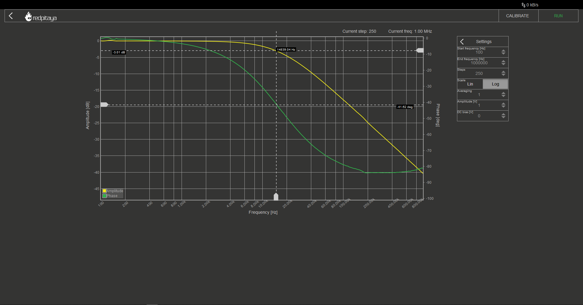
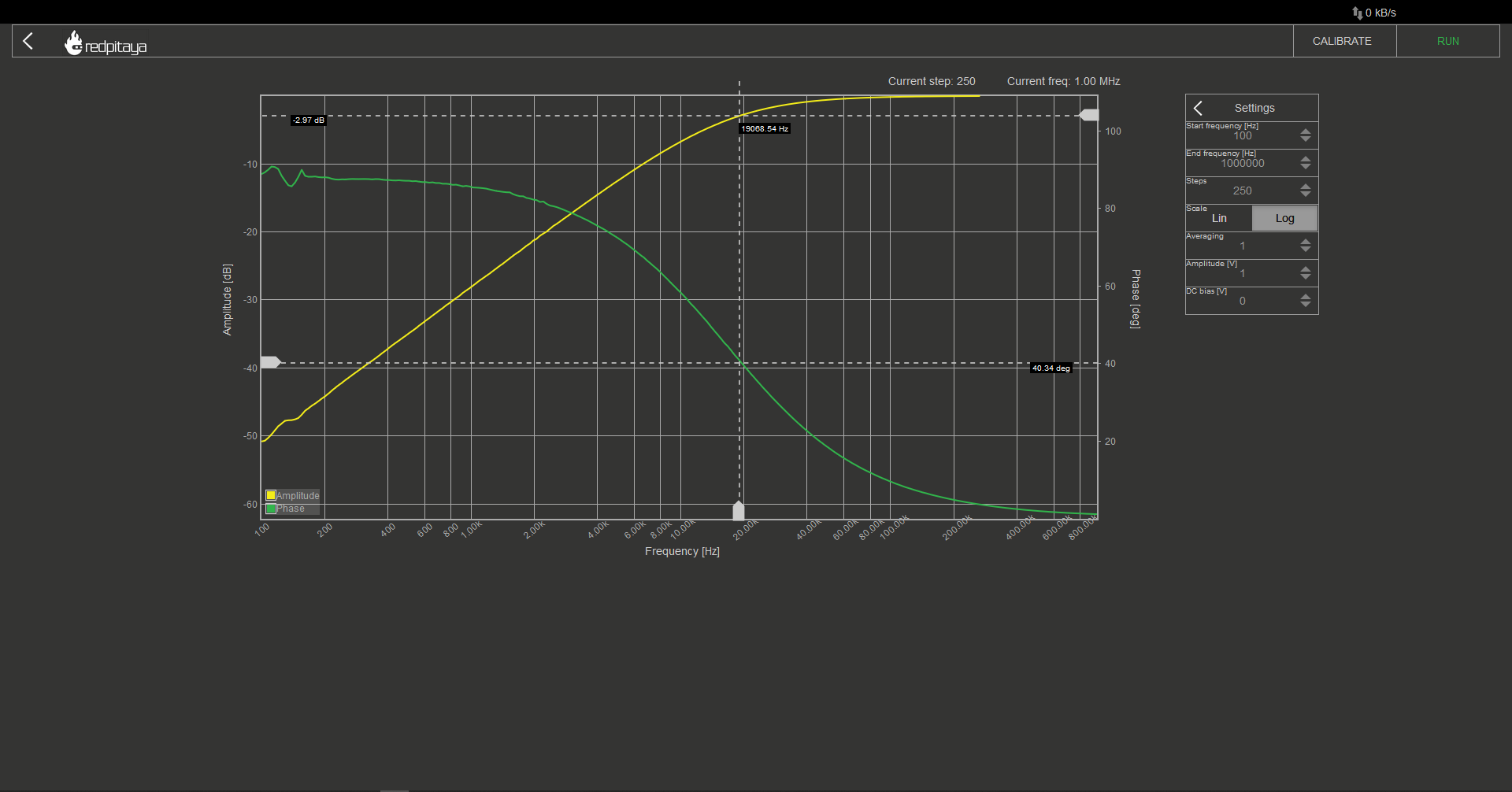
You will notice that this graph is quite a bit different than the idealized one. There are no sharp corners, corner frequency is too low, phase at corner frequency isn’t -45°, and it never reaches -90°. This isn’t even a comprehensive list of differences between ideal and real bode plot! Some differences can be attributed to idealized graph being oversimplified, some to component values having value tolerances, and some to parasitic properties of used components. Let’s not dwell on that and move on to a high pass filter. Just swap R and C and rerun the analysis.
It is important to note that the image does not explicitly state that the probes used in this setup must be in x1 mode and the signal output must have the lowest possible resistance. Using oscilloscope probes in place of a cable is not recommended for this purpose. To ensure proper calibration, the “calibrate” button on Red Pitaya’s bode analyzer can be used as a fail-safe measure.
Written by Luka Pogačnik Edited by Andraž Pirc
This teaching material was created by Red Pitaya & Zavod 404 in the scope of the Smart4All innovation project.