4.1. Using the Red Pitaya for measuring properties of periodic waveforms
4.1.1. Objective
This lab aims to use the Red Pitaya, a versatile tool for digital signal processing, to investigate various properties of periodic waveforms. We’ll demonstrate the functions of the Red Pitaya as an oscilloscope, signal generator, and spectrum analyzer, focusing on the measurement of waveform characteristics such as period, frequency, phase, and spectral content.
4.1.1.1. Period and Frequency of a Waveform
The period of a waveform is a crucial characteristic, defining the time it takes for one complete cycle of the wave to occur. It’s typically measured from peak to peak or trough to trough. The frequency, on the other hand, tells us how many of these cycles occur in one second. It’s typically measured in Hertz (Hz).
The Red Pitaya, in its capacity as an oscilloscope, is used in this lab to measure the period of a sinusoidal waveform. This can be achieved both manually, by using cursors to highlight a complete cycle on the oscilloscope’s display, and automatically, with the Red Pitaya’s built-in measurement capabilities.
Crucially, there is a simple mathematical relationship between the period (T) and frequency (f) of a waveform, expressed by the equation:
This equation highlights that the frequency is the reciprocal of the period, and vice versa.
4.1.1.2. Phase Difference
Phase difference is another vital characteristic of waveforms, particularly when comparing two or more signals. It refers to the difference in phase between two waveforms, represented as an angle (either in radians or degrees).
In this lab, we delve into the concept of phase difference by observing two 1500Hz sinusoids, one of which has been intentionally delayed by 45 degrees. This delay introduces a phase shift, which can be measured by observing the time difference between corresponding points (like peaks or zero crossings) on the two waveforms.
The phase difference (Φ) for signals of equal frequency can be calculated using the formula:
Here, Δt represents the time delay between the two waveforms.
4.1.1.3. Spectrum Analysis
The Red Pitaya is not just an oscilloscope, it’s also a potent spectrum analyzer. This functionality allows us to view the frequency content of a signal, showing how the signal breaks down into its constituent frequencies. This is achieved by performing a Discrete Fourier Transform (DFT) on the time-domain signal, converting it into the frequency domain.
The spectrum of a pure sinusoid will show a single peak at the sinusoid’s frequency. More complex waveforms, however, will have additional peaks representing the harmonic content of the signal. The power of these peaks can be measured in dBm, a logarithmic scale relative to a reference power of 1 milliwatt.
The conversion from a linear power scale (P_lin) to dBm is given by:
4.1.1.4. Comparing Waveforms in the Time Domain
This lab also provides a fascinating exploration of waveform analysis by comparing two waveforms in the time domain. We’ll investigate the effect of varying the amplitude, frequency, and phase of two waveforms displayed simultaneously on the oscilloscope.
The waveform pairs for comparison include: a sine and a cosine wave, a sine wave and a square wave, a sine wave and a sawtooth wave, and a sine wave and a pulse width modulated (PWM) output. These pairs are chosen to highlight the diverse features and behaviors of different types of waveforms. By manipulating the parameters of these waveforms and observing the resulting changes, we can gain a profound understanding of how these parameters affect the time-domain representation of signals.
In conclusion, this lab provides a practical and hands-on exploration of fundamental concepts in signal processing. The experiments showcase how to measure and analyze the characteristics of periodic waveforms using a versatile digital tool like the Red Pitaya
4.1.2. Goals of this Lab
Demonstrate ability to use Oscilloscope, Signal Generator, and Spectrum Analyzer capabilities of Red Pitaya through GUI.
Configure Red pitaya to receive external inputs.
Perform measurements on a multitude of periodic waveforms
4.1.3. Tasks / Measurements
Configure the Red Pitaya for a Loopback configuration (SMA cables tied between the outputs and inputs to the Red Pitaya) as shown in Fig. 1.
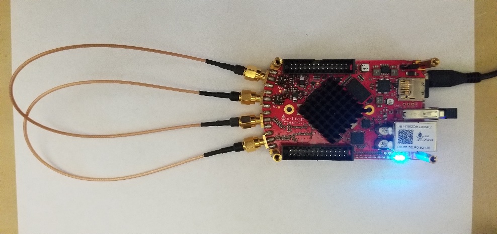
Fig. 1: Red Pitaya in Loopback Configuration
4.1.3.1. Measure the Period of a waveform – Time Domain
Open the Oscilloscope & function Generator Application.
Configure the output of the red pitaya for a 1500Hz Sinusoid as shown in Fig. 2.
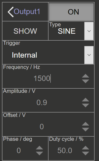
Fig. 2: OUT1 Configuration for measuring period/frequency
Configure the trigger for a negative edge trigger with zero level and normal trigger mode as shown in Fig. 3.
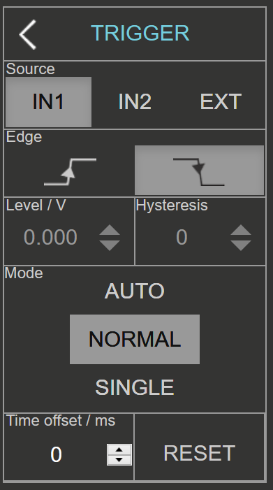
Fig. 3: Trigger Configuration
Enable OUT1. You should now see a figure close to the following
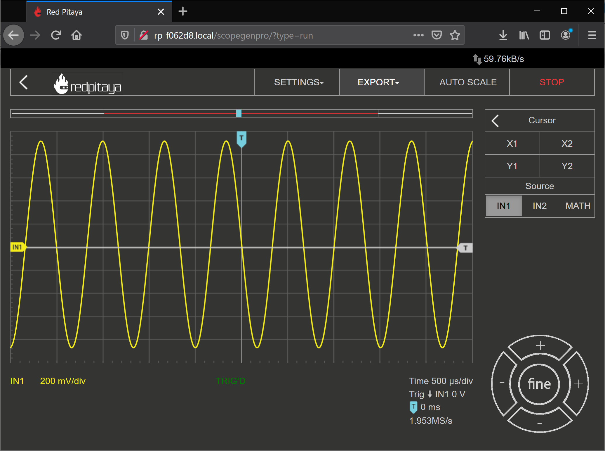
Fig. 4: Target output for 1500 Hz Sinusoid with negative edge triggering
To measure the period,
Select the “Cursor” box, and enable “X1”, “X2” options.
Drag each cursor to a common feature of the waveform (peak to peak, trough to trough)
Read off spacing between cursors. This is an approximate measure of the period
Period can also be measured by the red pitaya itself, under the meas command by selecting “Period” and “IN2”, and finally selecting “Done”. This is shown in Fig. 5.
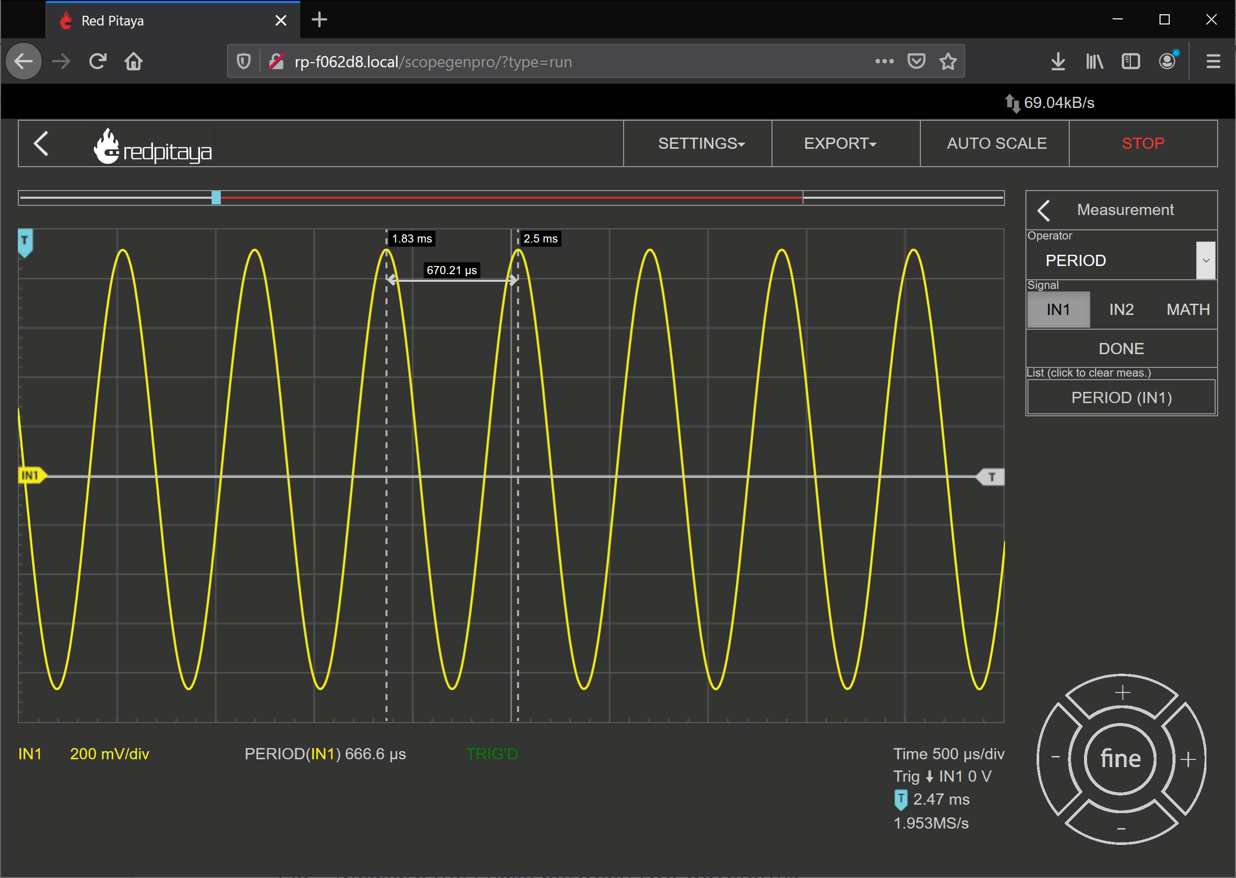
Fig. 5: Measured waveform vs Cursor measurement
4.1.3.2. Measure the Fundamental Frequency of a waveform – Time Domain
To measure the fundamental frequency of a waveform, bring up the X1,X2 cursors, and select a single period of the waveform. From there you can use the following relation to estimate the frequency of the waveform.:
to estimate the frequency of the waveform.
Once again, the Red pitaya can also calculate this by selecting the “FREQ” measurement option in the “Meas” options as shown below.
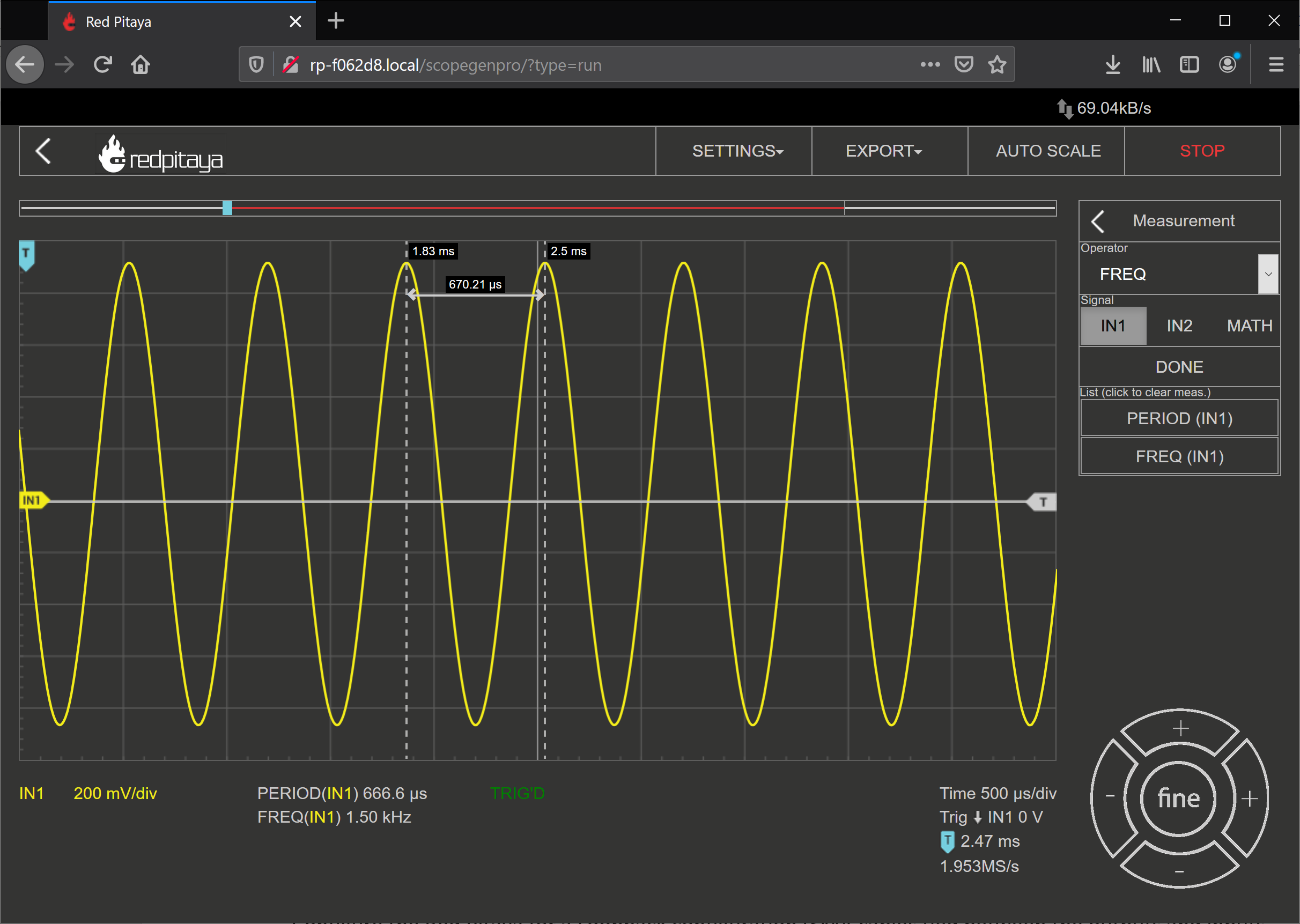
Fig. 6: Frequency Measurement added
4.1.3.3. Measure the Phase between two waveforms – Time Domain
Select output 2, and select the second output to be a 1500 Hz sine wave with a 45 degree phase shift
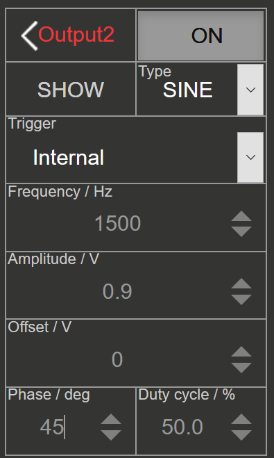
Fig. 7: Second channel configuration
Configure the trigger for a single shot acquisition as shown in Fig. 8.
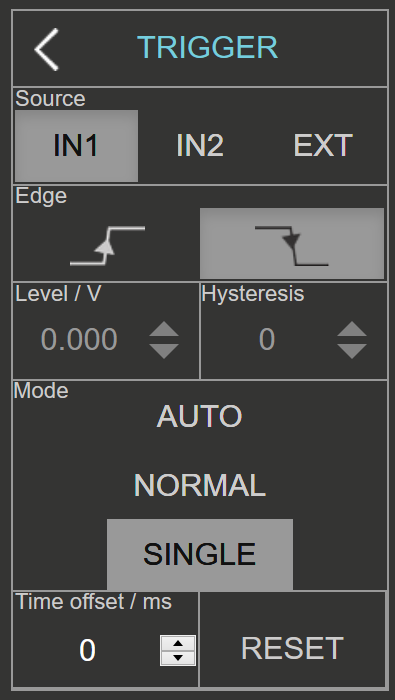
Fig. 8: Trigger configuration
Acquire a single capture, and measure the frequency and period of each waveform as previously described. Note that for the second channel, you may want to specify your cursors to track channel 2 in the cursor menu. To measure the Phase between waveforms, simply calculate the difference in time between two corresponding peaks between waveforms, and convert this to their corresponding difference in angular frequency. This can be calculated for signals of equal frequency with the relation
Analytically calculate the period of either waveform, and the time delay expected for the configured 45 degree phase shift between waveforms.
Set the output frequency of a OUT1 to 1000 Hz and trigger to normal or auto. What is the behavior that is observed? Comment as to the origin of the behavior, and a potential fix for the behavior. (hint,consider the greatest common divisor between the two frequencies)
(Take home) Repeat part 2, but for the frequency values of 3000Hz, and 1531Hz. What behavior is displayed here for each frequency? What are some potential ways to work around this problem? (hint, consider the greatest common divisor between the two frequencies, and alternative trigger modes)
4.1.3.4. Measure the Spectrum of the waveform - Frequency Domain
Open the DFT Spectrum Analyzer Application.
Recreate the waveform employed in 2.1. For convenience, this is reprinted below:
Configure the output of the red pitaya for a 1500Hz Sinusoid as shown in Fig. 2.
Set the Span of the spectrum analyzer to 6.5 kHz.
Observe the location of the peak(s), and infer what this implies about the sinusoid’s fundamental frequency and its purity (harmonic content). Mention the relative strength between the various peaks in dB and in linear scales, knowing the relation between dB and linear scales in dBm is given by:
4.1.3.5. Comparing Waveforms in the Time domain
Configure the Red Pitaya for a Loopback configuration (SMA cables tied between the outputs and inputs to the Red Pitaya) as shown in Fig. 1.
Reference Case: Sine and Cosine
Set OUT1 and OUT2 to be sines of the same frequency of 1000Hz, with equal amplitude. Set OUT2 to have a phase of 90 degrees.
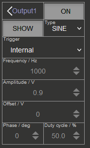
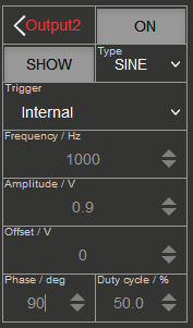
Fig. 9: Reference waveforms
Capture a screen shot of the resulting waveforms. Comment on any visible similarities or differences.
The two sine waves should look identical except for a phase shift. The wave on OUT2 should appear to start later than the wave on OUT1 because of the 90 degree phase shift.
Try varying amplitudes/frequencies/phases of both channels and comment on the overall effects each variable does as observed in the time domain. Capture a screen capture that demonstrates each observable change, and clearly label what change was done between each.
Changes in amplitude would cause the height of the waves to change. Changes in frequency would cause the waves to appear more condensed or expanded along the time axis. Changes in phase would cause the wave to appear to start earlier or later relative to the other wave.
(Take Home) Drop the amplitude of OUT2 to 0.45 V (0.5x amplitude). How much does the waveform’s Peak-to-Peak value change by?
When the amplitude is dropped to 0.45V, the peak-to-peak value should drop by half because the peak-to-peak value is essentially the amplitude of the signal.
4.1.3.5.1. Sine and Square
With the same setup as 2.5.1, change OUT1 to produce a SQUARE, as shown in Fig. 10.
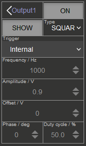
Fig. 10: OUT1 Configured for SQUARE output
Capture a screen shot of the resulting waveforms. Comment on and visible similarities or differences.
The sine and square waveforms will look significantly different. The sine wave is smooth and periodic while the square wave has abrupt changes and a flat peak and trough.
(Take Home) Try varying amplitudes/frequencies/phases of both channels and comment on the overall effects each variable does as observed in the time domain. Capture a screen capture that demonstrates each observable change, and clearly label what change was done between each channel. For any parameters that do not produce visible changes, comment on why you believe this is so.
Amplitude:
Frequency:
Phase:
Changes in amplitude, frequency, and phase will have similar effects as described in the sine-sine case. However, the square waveform will not have smooth transitions, and the changes may be more visually striking.
4.1.3.5.2. Sine and Sawtooth
With the same setup as 2.5.1, change OUT1 to produce a SAWU, as shown in Fig. 11.
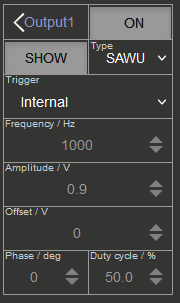
Fig. 11: OUT1 Configured for SAWU output
Capture a screen shot of the resulting waveforms. Comment on any visible similarities or differences.
The sine and sawtooth waves will also look quite different. The sine wave will still be smooth and periodic, while the sawtooth wave will have a linear increase and then an abrupt drop.
(Take Home) Try varying amplitudes/frequencies/phases of both channels and comment on the overall effects each variable does as observed in the time domain. Capture a screen capture that demonstrates each observable change, and clearly label what change was done between each channel. For any parameters that do not produce visible changes, comment on why you believe this is so.
Amplitude:
Frequency:
Phase:
As before, changes in amplitude, frequency, and phase will affect the height, spacing, and relative start time of the waves. Again, the sawtooth waveform will not have smooth transitions, and the changes may be more visually striking.
4.1.3.5.3. (Take Home) Sine and Pulse Width Modulated (PWM) output
With the same setup as 2.5.1, change OUT1 to produce a PWM, as shown in Fig. 12.
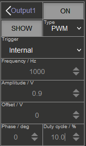
Fig. 12: OUT 1 configured for PWM output
Capture a screen shot of the resulting spectrums/spectrograms. Comment on any visible similarities or differences.
PWM waveform can look quite complex depending on its duty cycle. When combined with a sine wave, the differences could be substantial.
(Take Home) Try varying amplitudes/frequencies/phases of both channels and comment on the overall effects each variable does as observed in the frequency domain. Capture a screen capture that demonstrates each observable change, and clearly label what change was done between each channel. For any parameters that do not produce visible changes, comment on why you believe this is so.
Amplitude:
Frequency:
Phase:
Duty Cycle:
Changes in amplitude, frequency, and phase will continue to affect the waveforms as described. In addition, changes in duty cycle will alter the PWM waveform by changing the relative amount of time the signal is high versus low.
4.1.3.5.3.1. Inferences to be made / Questions
From the previous sets of measurements what instrument(s) would you use to measure each of the following quantities:
Amplitude:
The amplitude of a periodic waveform can be measured using an oscilloscope or a voltmeter. These instruments allow direct measurement of the voltage or signal level, providing an accurate measurement of the waveform’s amplitude.
Frequency:
The frequency of a periodic waveform can be measured using a frequency counter or a spectrum analyzer. These instruments analyze the waveform and determine the frequency content, providing an accurate measurement of the waveform’s frequency.
Phase:
The phase of a periodic waveform can be measured using an oscilloscope or a phase meter. These instruments compare the phase of the waveform with a reference signal and provide a measurement of the phase difference between them, indicating the waveform’s phase.
4.1.3.5.3.2. Conclusion
The lab exercise provides a hands-on exploration of waveform analysis using the Red Pitaya, a versatile digital signal processing tool. Throughout the lab, we demonstrated how the Red Pitaya functions as an oscilloscope, signal generator, and spectrum analyzer to examine key properties of periodic waveforms including their period, frequency, phase, and spectral content. The comparative analysis of different waveform pairs in the time domain showcased the impact of varying amplitude, frequency, and phase. Notably, the Red Pitaya’s spectrum analyzer capability allowed us to visualize and understand the harmonic content of complex waveforms. Ultimately, this lab experience underpins the profound understanding of signal processing concepts and bolsters the ability to perform comprehensive waveform measurements and analysis.
4.1.3.5.3.3. Reference text
For more in-depth documentation, view the official documentation at: