4.5. Brief Tour of Nonlinear Systems
4.5.1. Introduction
The purpose of this lab is to perform analysis on simple non-linear systems, measure frequency responses for these systems, and demonstrate their use-cases. Nonlinear systems differ from Linear Time Invariant (LTI) systems as they do not follow the principles of linearity and superposition. They exhibit non-linear behavior and do not have sinusoids as eigenfunctions. In this lab, we will explore the effects of non-linear systems and analyze their frequency responses.
4.5.2. Nonlinear Systems
4.5.2.1. Definition and Characteristics
Nonlinear systems are mathematical models that do not adhere to the principles of linearity and superposition. These systems exhibit complex relationships between the input and output variables, often involving non-linear equations. Unlike linear systems, the response of a nonlinear system is not directly proportional to the input and cannot be expressed as a sum of independent responses.
4.5.2.2. Departure from Linearity and Superposition
Linearity is the property of a system where the output is directly proportional to the input. Superposition states that the response to a sum of inputs is equal to the sum of individual responses. Nonlinear systems violate these principles as their behavior is governed by nonlinear equations. The output of a nonlinear system depends on the interaction of multiple inputs, and the response is not simply additive or proportional.
4.5.2.3. Nonlinear Equations and Models
Nonlinear systems can be described by non-linear equations that involve terms with powers, exponentials, logarithms, or other non-linear functions. These equations may not have closed-form solutions or may require numerical methods for analysis. Nonlinear models are used to represent various physical, biological, and engineering systems, including electrical circuits, chemical reactions, biological processes, and economic systems.
4.5.3. Diodes
Diodes are a semiconductor device that is formed by a PN junction. The current-voltage (I-V) relation of the device can be described by the Ideal (Shockley) diode equation:
Where \(K_{B}\) is the Boltzmann constant, \(T\) is the temperature in Kelvin, \(q\) is the absolute value of the charge of an electron in Coulombs, and \(I_{0}\) is the reverse saturation current in amperes. When \(V \ll K_{B}T/q\), the argument to the exponent becomes very small, and \(\exp\left( \frac{V}{K_{B}T/q} \right) \ll 1\). This makes \(I \approx \ - I_{0}\). Conversely, when \(V \gg K_{B}T\)/q, \(\exp\left( \frac{V}{K_{B}T/q} \right) \gg 1\), and thus \(I \approx I_{0}\exp\left( \frac{V}{K_{B}T/q} \right)\). This exponential relationship is obviously non-linear, and can be made explicit by taking the taylor series of the exponential function:
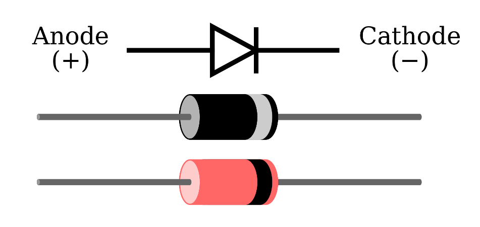
This nonlinear behavior can be exploited for many applications. The diode symbol is shown below, and has an anode and cathode ends. This is reflected in the package by a stripe on the end of the package that mirrors the line in the diode symbol.
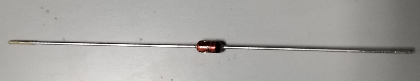
1n914 diode with Cathode bar on right
4.5.4. Linearization of Nonlinear Systems
4.5.4.1. Linearization Principles and Techniques
Linearization is a process that approximates the behavior of a nonlinear system around a specific operating point by using linear models. It involves finding the tangent or linear approximation of the nonlinear function at the operating point. The linearized model provides a simplified representation that enables the application of linear analysis techniques and tools.
Linearization is based on the concept that for small deviations from the operating point, the nonlinear function can be approximated by its linear behavior. This is possible by considering the first-order terms of a Taylor series expansion. The Taylor series expansion represents a nonlinear function as a sum of terms that capture the behavior of the function at different orders of deviation from the operating point.
4.5.4.2. Approximation of Nonlinear Functions by Linear Functions
To perform linearization, the nonlinear function is approximated by a linear function with a constant term and a linear term that represents the deviation from the operating point. The constant term represents the value of the function at the operating point, while the linear term captures the effect of small deviations from the operating point.
The linear approximation is obtained by truncating the Taylor series expansion after the first-order term. This is justified when the deviations from the operating point are small enough that higher-order terms can be neglected. By retaining only the linear term, the nonlinear function is effectively replaced by a linear function, allowing for the use of linear analysis techniques.
The linearization process involves the following steps:
Choose an operating point: Select a specific point around which the linearization will be performed. This point should be representative of the system’s behavior and provide a good approximation of the nonlinear function.
Compute the partial derivatives: Calculate the partial derivatives of the nonlinear function with respect to each input variable at the operating point. These derivatives represent the sensitivity of the function to changes in each input variable.
Formulate the linear approximation: Using the partial derivatives, construct the linear approximation of the nonlinear function. The constant term is the value of the function at the operating point, and the linear term is the sum of the partial derivatives multiplied by the deviations from the operating point.
Validate the linear approximation: Assess the validity of the linear approximation by comparing it to the original nonlinear function. This can be done by evaluating the approximation at different points and comparing the results to the true nonlinear function.
Linearization provides a useful tool for simplifying the analysis of nonlinear systems. By approximating the nonlinear behavior with a linear model, it becomes possible to leverage the extensive theory and techniques developed for linear systems. This enables the application of various linear analysis methods, such as frequency response analysis, stability analysis, and control design, to gain insights into the behavior of the nonlinear system.
4.5.5. Hands on experiment
Connect the cables to the Red Pitaya via the adapters as shown in Fig. 1, noting that we need IN1,IN2, and OUT1 connections.
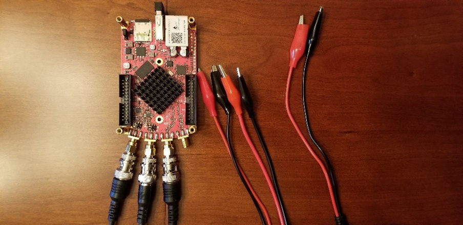
Fig. 1: Red Pitaya hardware configuration
4.5.6. Tasks / Measurement
4.5.6.1. Half bridge rectifier
Build the Single stage RC circuit shown in Fig. 2, with \(R = 10k\Omega\),\(D = 1N914\).
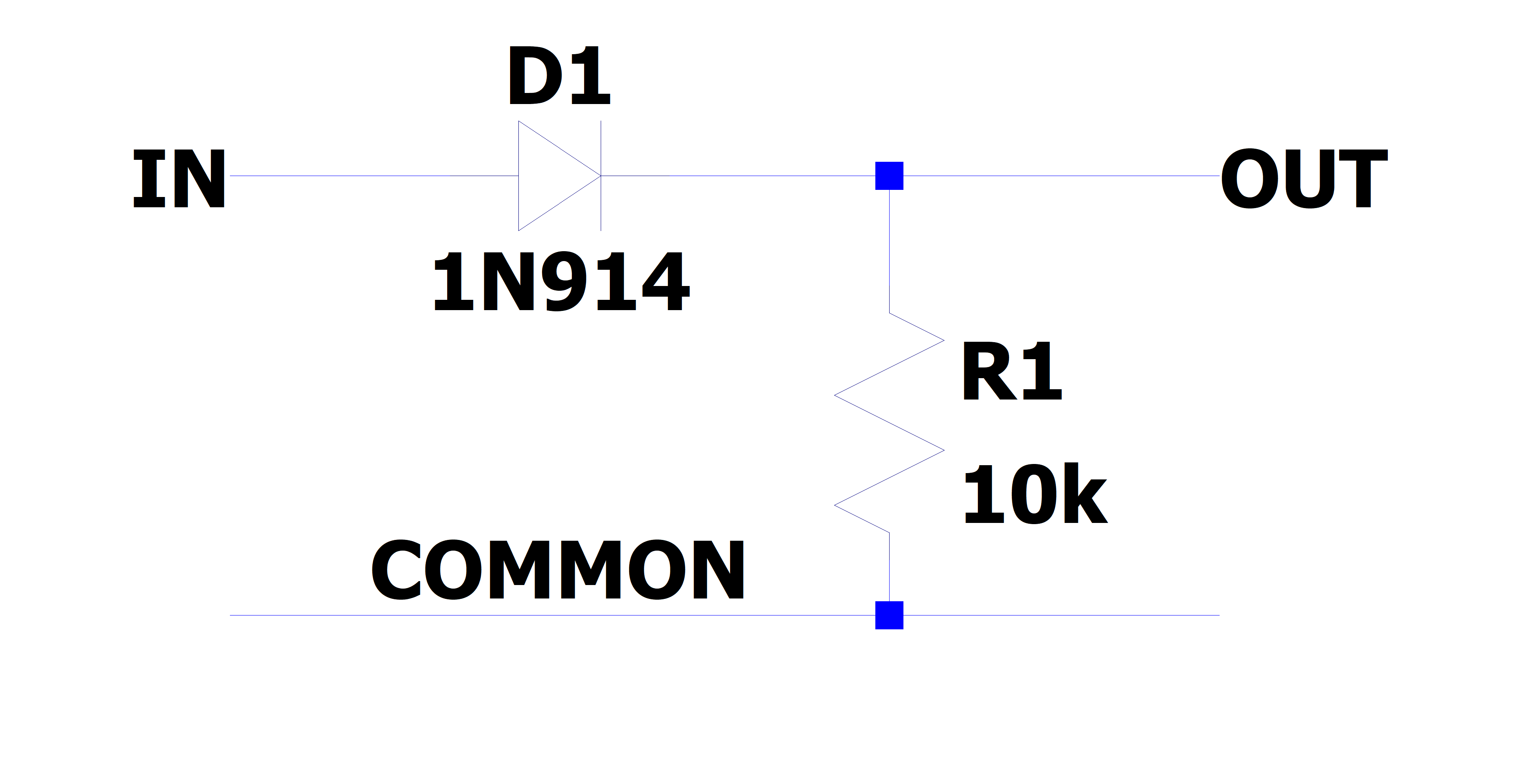
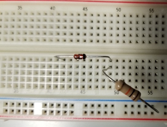
Fig. 2: (left) schematic of the single stage RC circuit, (right) implementation on breadboard
4.5.6.1.1. Analysis
Oftentimes in analysis for a nonlinear systems, we choose to linearize the system about a specific operating point. This leverages the fact that for a small perturbation \(V_{new} = V_{old} + \delta V\), the series expansion of a nonlinear function will be primarily linear for small \(\delta V\). This comes from the calculation of the powers of \(V_{new}\); for instance,
If \(2\delta V \ll \ V_{old}\), then
where \(\epsilon\) is some error term. Applying the same logic to the ideal diode equation gives us the response.
Rearranging to subtract out the original current \(I\),
Calling \(\frac{V}{K_{B}T/q} = V_{0},\frac{\delta V}{K_{B}T/q} = V_{\delta}\)
Applying a Taylor expansion on all terms
Cancelling like terms being subtracted in the brackets gives
Finally applying the approximation \(\left( V_{0} + V\_\delta \right)^{2} \approx \left( V_{0} \right)^{2}\) and cancelling the resulting terms
At this point, the perturbation can be make to look like ohm’s law, and thus the perturbation is linear in behavior. This is equivalent to approximating the I-V curve of the diode as a tangent line approximation, and is a theme that is used extensively in engineering and applied mathematics.
Using the above linearization, what does the frequency response of the half bridge circuit look like?
After linearization, we can treat the diode as a resistor. As a result, the diode and resistor act together as an RC filter, and the frequency response would be similar to an RC high-pass filter. This is because the diode and resistor together (R_D) forms an RC circuit with the capacitor.
4.5.6.1.2. Measurement
Using the Red Pitaya’s Bode Analyzer tool, measure the frequency response (\(\left| T(f) \right|\)) as described in the previous lab. Keep in mind that for this circuit, we stated that the amplitude must be small. Set the DC bias to > 0.6V to ensure the diode is forward biased while testing.
Show the plot of the measurement below:
Try making the amplitude larger and see what occurs. Find a point at which the behavior is no longer linear
Using the Red Pitaya’s Bode Oscilloscope & Spectrum analyzer tools, measure the large signal response to a sinusoid:
With DC Bias of 0.7V, and amplitude 0.1
In this scenario, the diode is forward-biased because of the DC Bias of 0.7V which is greater than the threshold voltage of the diode (typically around 0.6V for silicon diodes like the 1N914). The amplitude of 0.1 is relatively small, and hence you will mostly see a sinusoidal output but there may be some small distortion due to the diode’s non-linear characteristics.
With DC bias of 0V, and amplitude 1V
In this case, there is no DC bias and the signal’s amplitude is large (1V), exceeding the diode’s forward voltage. The diode will start conducting when the input voltage is positive (creating a positive half-wave), but will block current when the input is negative. The output will therefore be a half-wave rectified sinusoidal wave, showing only the positive half-cycles of the input.
Comment on the Spectral content of the output signal when compared to the input signal.
The spectral content of the output signal will include the fundamental frequency and harmonics when compared to the input signal, due to the non-linearity of the diode.
Show a plot of the both the time waveforms and frequency domain.
4.5.6.1.3. Comparison
Respond to the following questions:
Find the -3dB point in the circuit, and compare this value to the one you previously calculated.
The -3dB point can be found from the frequency response plot by finding the frequency at which the gain drops to approximately 70.7% of the maximum value.
4.5.7. Conclusion
In this lab, we explored the concepts and characteristics of nonlinear systems. We discussed the behavior of diodes and their nonlinearity, as well as the linearization techniques used to approximate the behavior of nonlinear systems. Through practical measurements and analysis of a half bridge rectifier circuit, we investigated the frequency response and the effects of amplitude variation. The comparison of spectral content and the examination of time waveforms and frequency domains provided insights into the behavior of the circuit. By studying nonlinear systems, we gain a deeper understanding of their unique properties and applications in various fields.