4.4. Measuring the Frequency response of LTI Systems with the Red Pitaya
4.4.1. Goals of this lab
In this course, our primary objective in the lab is to delve deeply into the realm of Linear Time-Invariant (LTI) systems. We will embark on a comprehensive exploration, combining theoretical analysis, practical measurements, parameter estimation, and demonstrations to gain a thorough understanding of the frequency responses exhibited by these systems. Additionally, we will examine their application in evaluating real-world components, and elucidate the intriguing concept of LTI system stacking.To commence this educational journey, we will engage in meticulous analysis of simple LTI systems.
4.4.2. Theory
4.4.2.1. LTI systems
In general, a Linear system is a system that takes and input \(X\), and produces an output \(Y\), that can be defined by a series of linear operators. Recall a linear operator is an operation that satisfies the principles of scalar multiplication and superposition. More mathematically, for vectors \(\mathbf{x,y}\), scalars \(\alpha,\beta\), the operator \(A\) is linear if:
is satisfied. Examples of linear operators are:
Differentiation/Integration
Convolution
Gradient/Divergence/Curl
Laplace/Fourier transforms
Note that if there are multiple Linear systems, their cascaded effect can be described by composing each subsequent system with the output of the other. This is equivalent to combing each of the operators the systems are implementing and forming a compound operator.
Time invariance is the property that for a given system, if \(y(t)\) is the output of the system when given an input \(x(t)\), then applying a delayed input \(x(t - T)\) will produce \(y(t - T)\), a delayed version of \(y(t)\). In the Time domain, this system has an impulse response \(h(t)\) and relates \(y(t)\),\(x(t)\) by the relation:
Where \(*\) is the convolution operation. The act of convolution can be difficult, so it is oftentimes more convenient to operate in another domain through some sort of transformation. A common transform is the Fourier transform, whereby a time domain signal is represented in the frequency domain. A consequence of the transform is the convolution operation is now reduced to multiplication.
Where \(H(f)\) is now the transfer function or frequency response of the system. Canonically, the transfer function is written as:
Every LTI system can be described by a given transfer function, with various systems being formed by various coefficients \(a,b\). In this lab, we will form a small number of systems with real components, and examine their behaviors.
4.4.2.2. Transfer Function
The transfer function is a fundamental concept in the analysis and design of linear time-invariant (LTI) systems. It represents the relationship between the input and output signals of a system in the frequency domain. By examining the transfer function, we can understand how the system processes different frequency components of the input signal. It captures the system’s frequency response characteristics, such as amplification, attenuation, and phase shifts.
Mathematically as mentioned above, the transfer function, denoted as H(f), is defined as the ratio of the output signal Y(f) to the input signal X(f):
The transfer function is obtained through the Fourier transform of the system’s impulse response, simplifying the analysis of the system’s behavior. It is typically expressed as a rational function of complex variables, with the numerator and denominator represented by polynomials. This allows us to determine the system’s gain and phase response. Understanding the transfer function enables engineers and researchers to design LTI systems with desired frequency response characteristics, optimizing their performance for specific applications. By leveraging the transfer function, we can accurately analyze and predict how a system amplifies or attenuates specific frequencies and introduces phase shifts. This knowledge is invaluable for tailoring the system’s behavior to meet the desired requirements.
4.4.2.3. Types of Filters
Filters are LTI systems used to modify the frequency content of a signal. They can be classified into different types based on their frequency response characteristics. A low-pass filter allows frequencies below a certain cutoff frequency to pass through while attenuating higher frequencies. It is commonly used to remove high-frequency noise and retain the low-frequency components of a signal. A high-pass filter, on the other hand, allows frequencies above a certain cutoff frequency to pass through while attenuating lower frequencies. It is useful for extracting high-frequency information and eliminating low-frequency noise. A band-pass filter allows a specific range of frequencies to pass through while attenuating frequencies outside that range. It finds applications in tasks such as signal isolation and frequency selection. Finally, a band-stop filter, also known as a notch filter, attenuates a specific range of frequencies while allowing other frequencies to pass through. It is effective in removing unwanted frequency components or interference.
4.4.2.4. Frequency Response
The frequency response of a linear time-invariant (LTI) system provides crucial insights into its behavior across different frequencies. It characterizes how the system processes and modifies signals of varying frequencies. The frequency response consists of two components: the magnitude response and the phase response.
The magnitude response represents the system’s gain or attenuation for each frequency component. It quantifies how much the system amplifies or attenuates different frequencies in the input signal. Mathematically, the magnitude response is denoted as
where
is the transfer function of the system. By examining the magnitude response, we can understand how the system enhances or diminishes specific frequency components, thereby shaping the overall spectral content of the output signal.
The phase response, on the other hand, reveals the phase shift introduced by the system at each frequency. It indicates the time delay or advance experienced by different frequency components of the input signal. The phase response is denoted as
and is essential for applications where phase synchronization or time relationships between signals are critical. By analyzing the phase response, we can determine the phase characteristics of the system and how it influences the timing of the output signal relative to the input signal at different frequencies.
Both the magnitude and phase responses are typically plotted as functions of frequency to visualize their characteristics. These frequency response plots provide valuable information about the system’s behavior, such as frequency selectivity, gain variations, and phase distortions. They serve as a powerful tool for analyzing and designing systems in various fields, including signal processing, communication, audio engineering, and control systems.
4.4.2.5. Impulse Response
In the time domain, the impulse response of an LTI system is a key concept for understanding its behavior. It characterizes the system’s response when the input signal is an impulse function, often represented as :math:h(t). The impulse response provides valuable insights into how the system processes signals over time and shapes the output signal based on its inherent properties. Mathematically, the output signal :math:y(t) of an LTI system can be obtained by convolving the input signal :math:x(t) with the impulse response :math:h(t) as expressed by the integral equation:
This equation represents the superposition of the weighted contributions of the input signal at different time instances, where the weights are determined by the impulse response. The impulse response reveals the system’s temporal characteristics and provides information about its response to instantaneous changes in the input signal. By examining the impulse response, we can understand phenomena such as signal distortion, time-domain filtering, and transient behavior of the system.
4.4.2.6. Stability
Stability is a fundamental property of LTI systems that ensures their reliable and predictable operation. A stable system maintains a bounded output for bounded input signals, providing confidence in its performance and behavior. Stability analysis is crucial in evaluating the robustness and reliability of LTI systems. The stability of an LTI system can be determined by examining its transfer function or impulse response. Various stability criteria, such as the location of poles in the complex plane or the boundedness of the impulse response, are employed to assess stability. A stable system exhibits desirable characteristics, such as controlled response to inputs, absence of oscillations, and suppression of noise and disturbances. In contrast, an unstable system may exhibit erratic behavior, uncontrollable oscillations, or even diverging responses. Ensuring stability is of utmost importance in the design and analysis of LTI systems. It enables reliable signal processing, accurate control systems, and effective communication.
By analyzing the stability of an LTI system, we can gain insights into its performance limitations and make informed decisions in system design and implementation. Stability considerations become particularly crucial in applications where precision, robustness, and error-free operation are essential. Stable LTI systems have widespread applications in various fields, including control systems, telecommunications, audio processing, and image processing. They provide a foundation for designing systems that exhibit desired behaviors, such as accurate signal reproduction, noise suppression, and precise control of dynamic processes. Stability analysis allows engineers and researchers to ensure the reliability and safety of LTI systems in real-world scenarios, where external disturbances, noise, and uncertainties may be present.
Furthermore, stability analysis plays a pivotal role in stability-based control design. Controllers are designed to stabilize unstable systems or improve the stability margins of marginally stable systems. Stability analysis techniques help identify the critical parameters and system characteristics that affect stability, guiding the selection and adjustment of control parameters to achieve desired stability and performance objectives.
In summary, understanding and analyzing the stability of LTI systems is crucial for ensuring their reliable operation, robustness, and optimal performance. Stability considerations guide system design, control design, and decision-making processes in various engineering disciplines. By evaluating the stability characteristics of LTI systems, engineers and researchers can create systems that meet performance requirements, mitigate undesirable effects, and deliver reliable and predictable results in diverse applications.
4.4.2.7. Materials
For this lab, you will need:
1x Red Pitaya
3x SMA to BNC adapters
3x BNC to alligator clamp cables
1x Breadboard
1x package of passive components
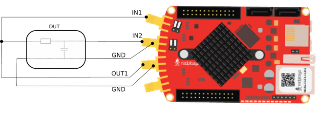
Connect the cables to the Red Pitaya via the adapters as shown in Fig. 1, noting that we need IN1,IN2, and OUT1 connections.
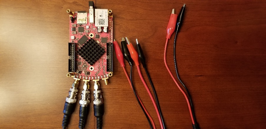
Fig. 1: Red Pitaya hardware configuration
4.4.2.8. A quick introduction to Breadboards and Passive components
4.4.2.8.1. Breadboards
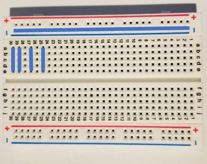
Bread boards are arrays of metal contacts internally tied together on a row wise basis (a,b,c,d,e) that are electrically separated on the columns (1,2,3,…,30). The exception to the rules are the bus bars on the extreme sides of the breadboard, where the entire row of the (-,+) rows are all electrically connected together. This is useful when using common terminals that are used through the circuit (as in the case of common, ground, or power supply nodes.
4.4.2.8.2. Passives
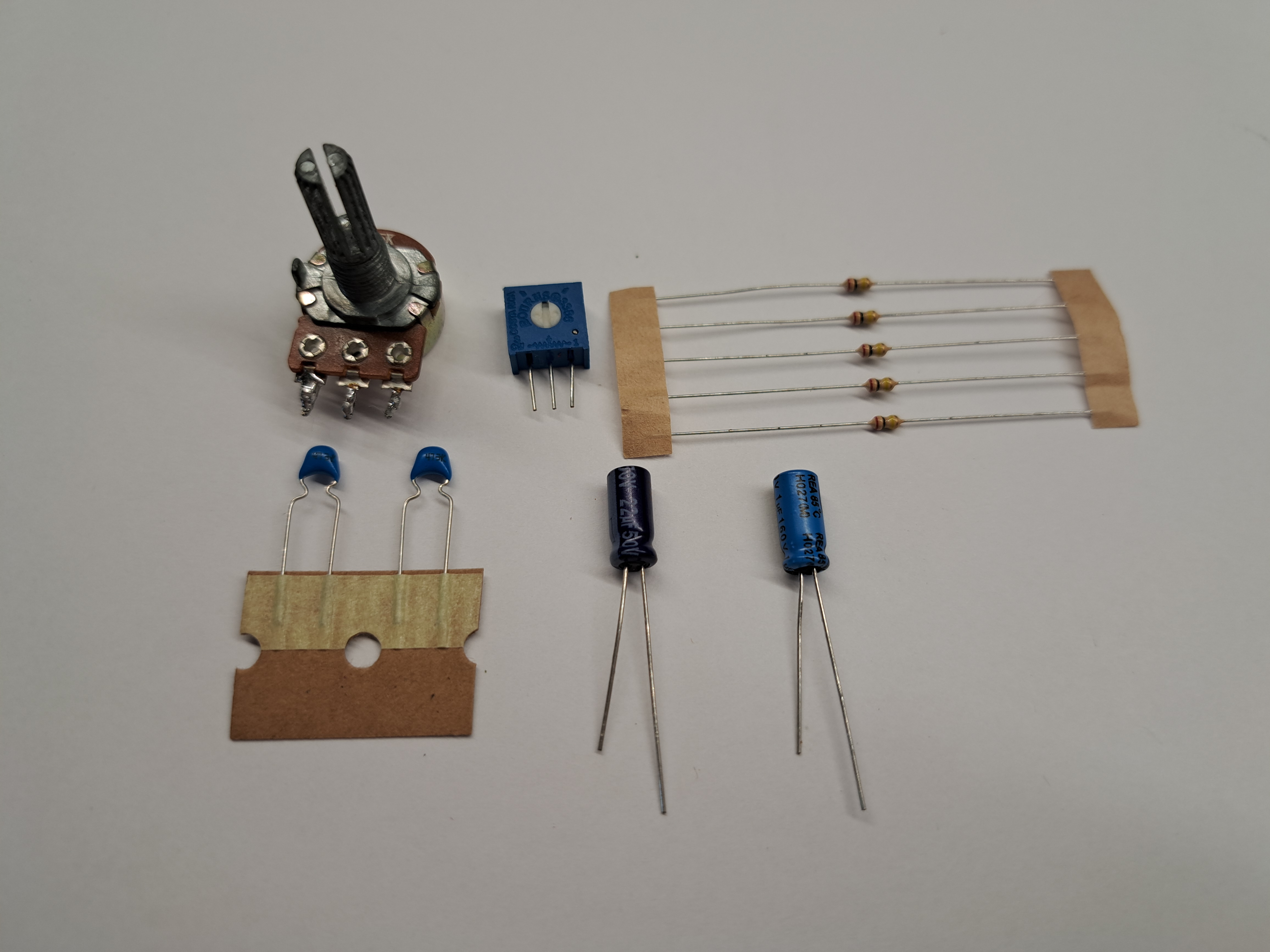
4.4.2.8.3. Resistors
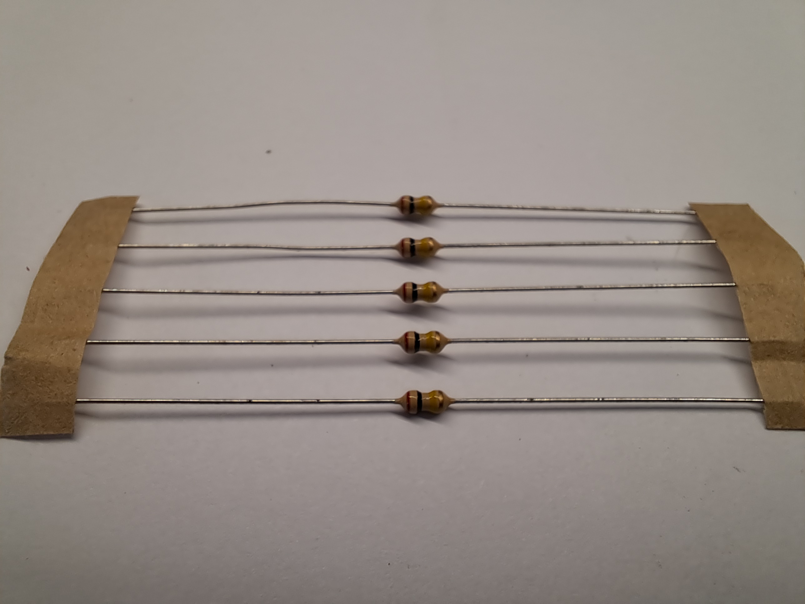
Resistors are a general element that obey Ohm’s law:
Where \(R\) is the resistance measured in Ohms (V/A) is a measure of the resistance to current flow. These are frequency independent devices.
4.4.2.8.4. Capacitors
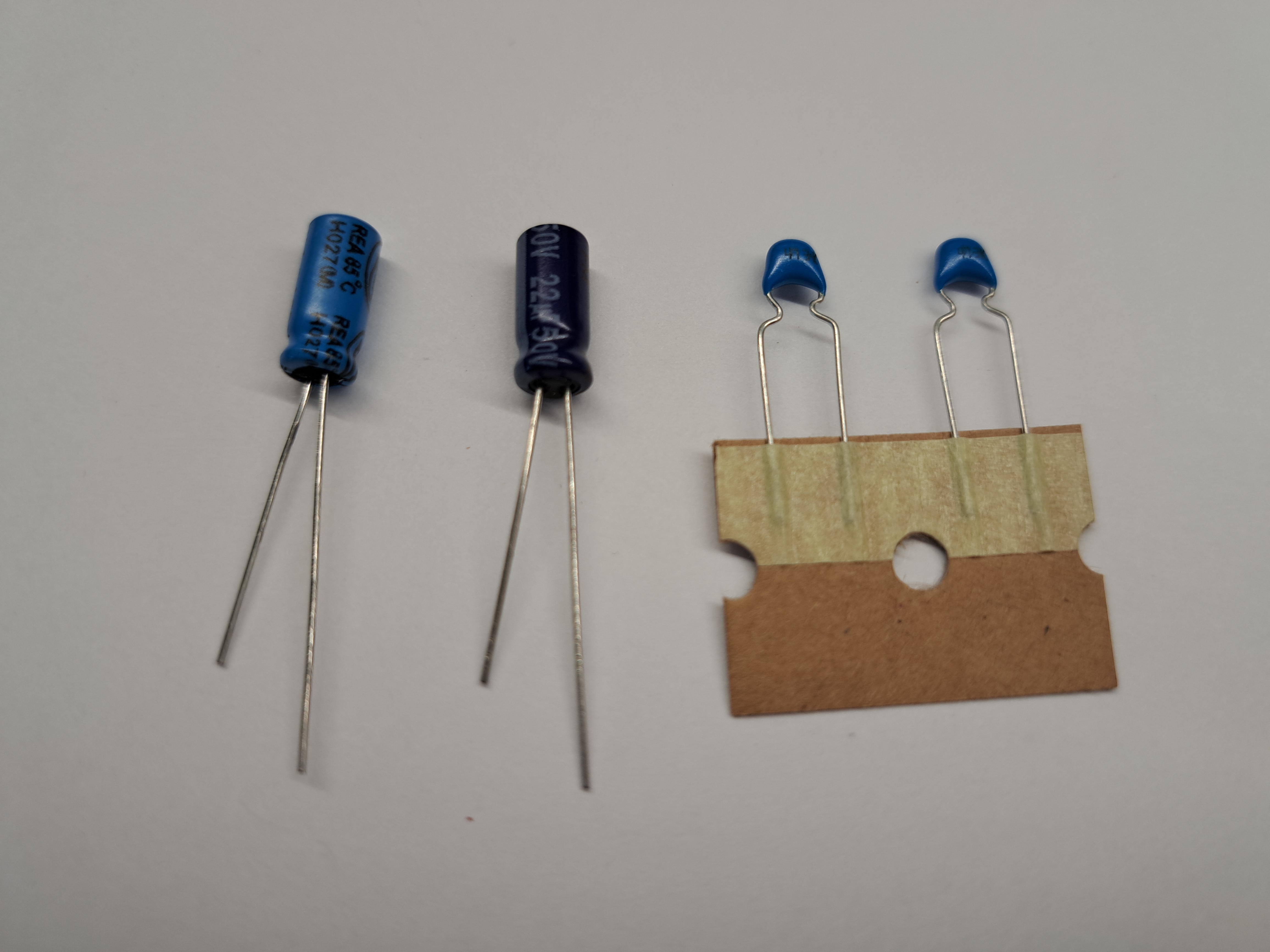
Capacitors have the Current-voltage relation:
Where \(C\) is the capacitance measured in Farads (V/m). Capacitors have the impedance:
4.4.2.8.5. Potentiometers
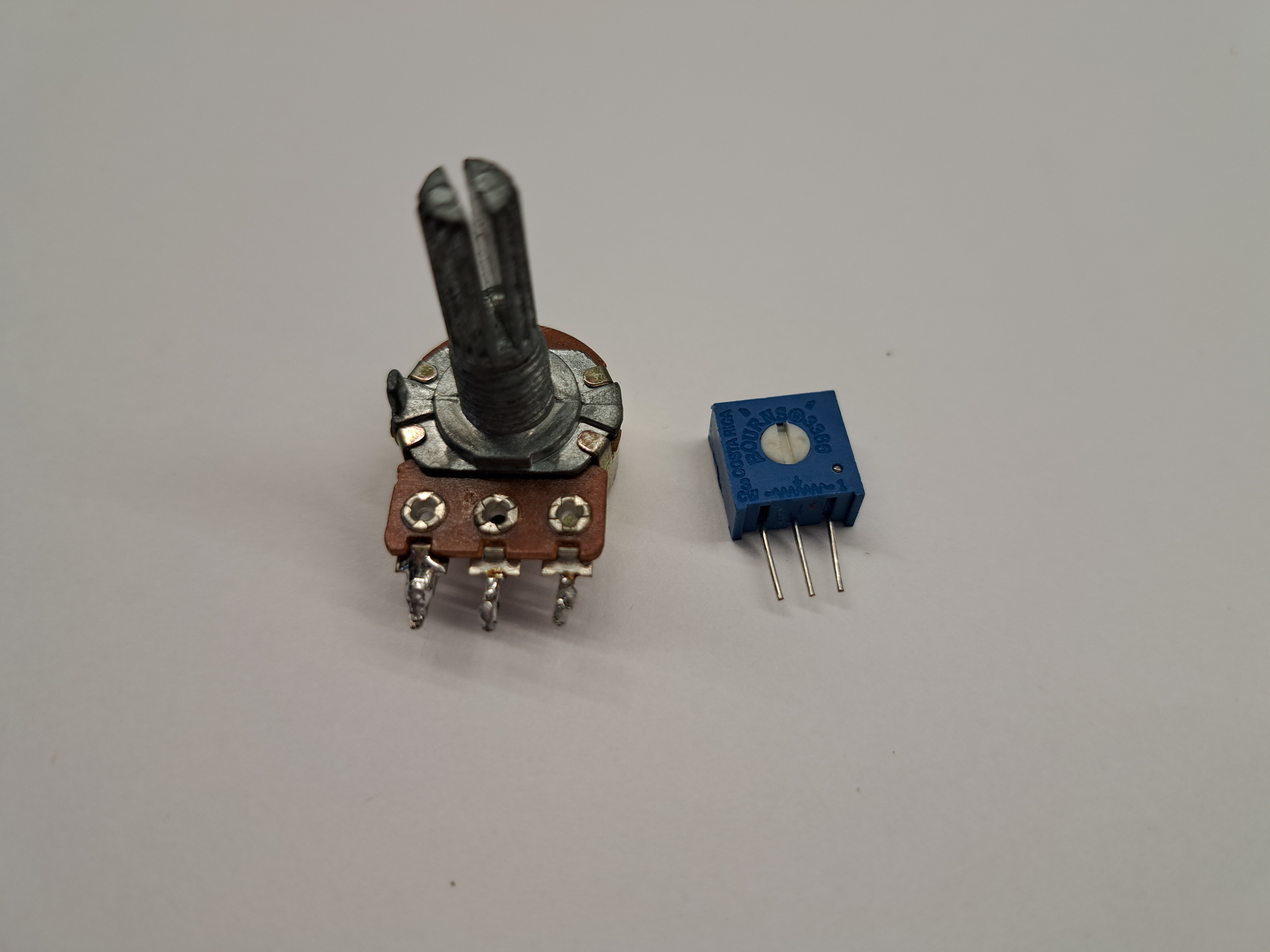
Potentiometers are three terminal devices consist of a resistor and a sliding contact that effectively breaks the resistor into two separate resistances. Depending on the contact location, the proportion of the total potentiometer resistance is distributed to each branch.

4.4.3. Tasks / Measurements
4.4.3.1. Single stage RC circuit – 1
Build the Single stage RC circuit shown in Fig. 2, with \(R = 10k\Omega\),\(C = 0.47\mu F\).
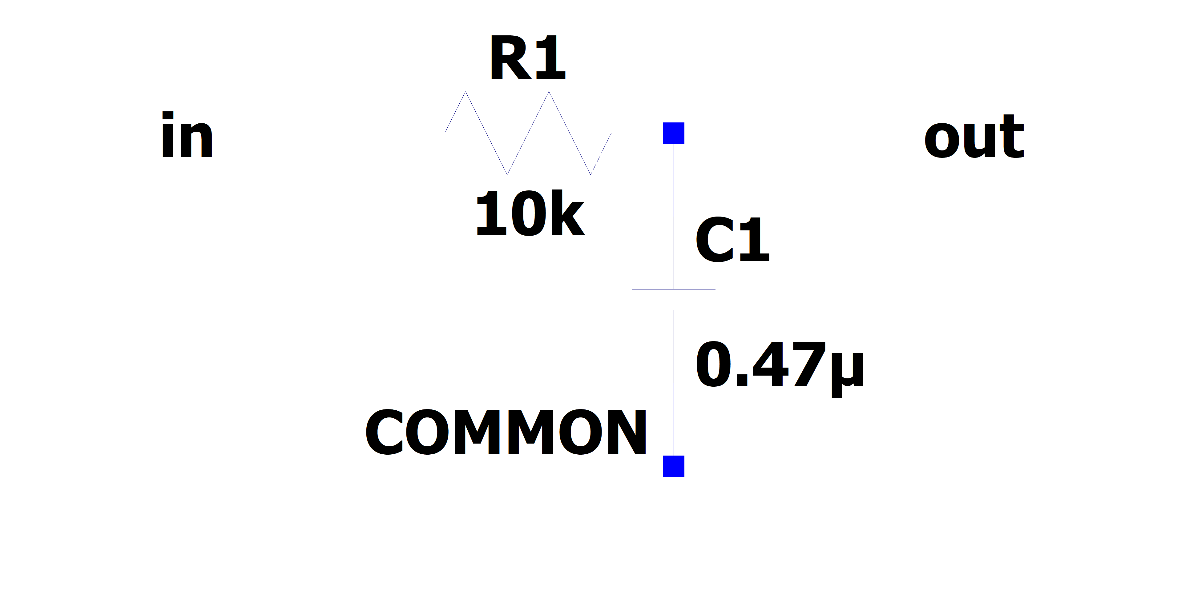
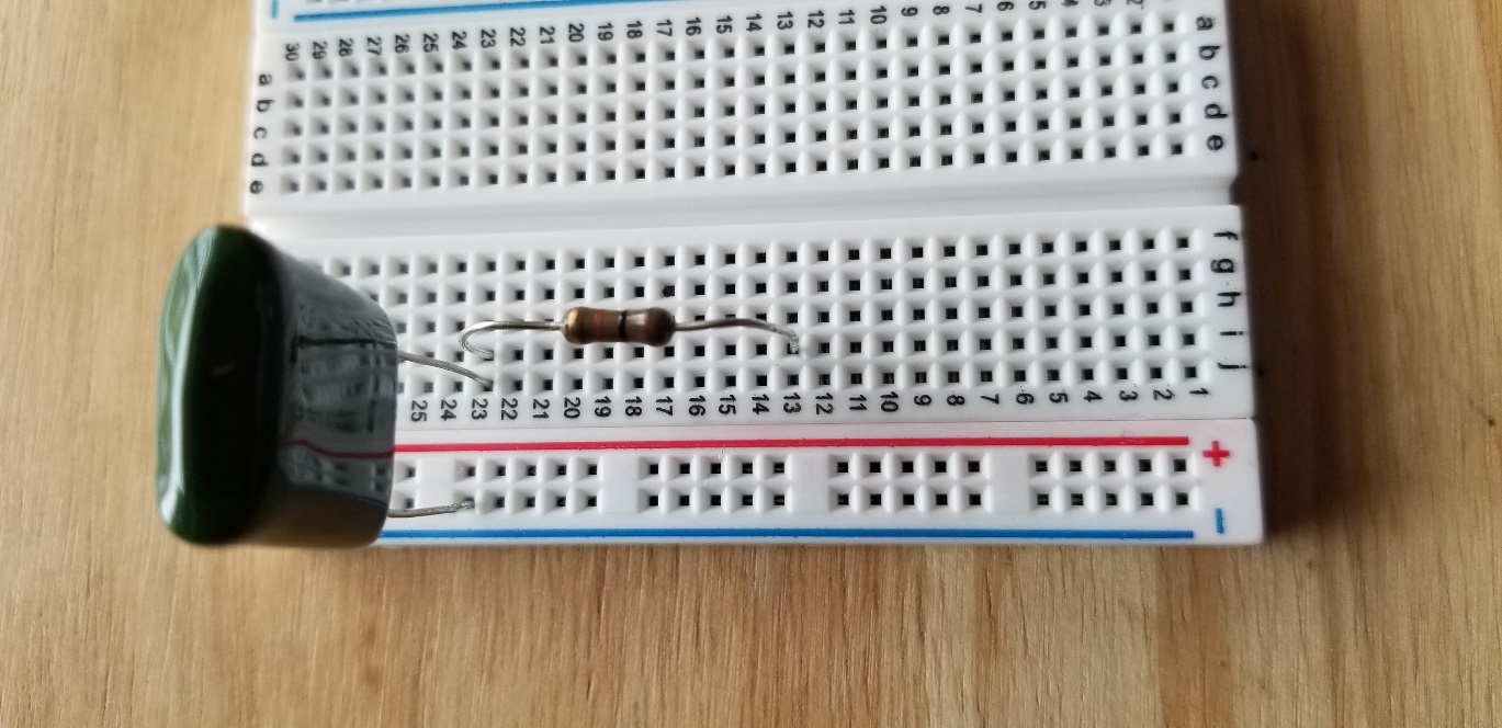
Fig. 2: (left) schematic of the single stage RC circuit, (right) implementation on breadboard.
4.4.3.1.1. Analysis
The claimed transfer function of this circuit is
Where \(j = \sqrt{- 1}\) is the imaginary unit.
What is the magnitude of the transfer function?
What is the phase response of the circuit?
What class (low-pass, high-pass, band-pass, band-stop) of filter is this? (This is equivalent to asking what happens to \(\left| T(f) \right|\) as \(f\) gets lower or higher?)
At what frequency does \(\left| T(f) \right| = \frac{1}{\sqrt{2}} \approx 0.707\)? (This corresponds to the so-called “half power point” where the ratio of the input to output power is 2 (-3dB) – The circuit drops half of the total power) This value is generally referred to the “cutoff frequency” or “-3dB frequency” and is represented by \(f_{c}\).
- (optional) What would happen if I swapped the input and output ports?(Hint: is there any current flowing through the resistor?)
4.4.3.1.2. Measurement
Using the Red Pitaya’s Bode Analyzer tool, measure the frequency response (\(\left| T(f) \right|\)).
Connect the Red Pitaya to the circuit, also known as the Device Under Test (DUT)), as shown below
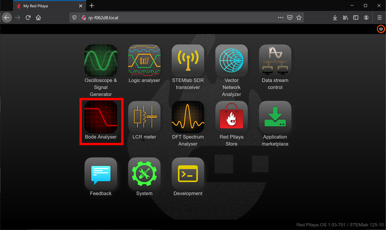
Connect to the Red Pitaya and select the Bode Analyzer tool.
A more detailed description of the Bode analyzer can be found here: Bode Analyzer
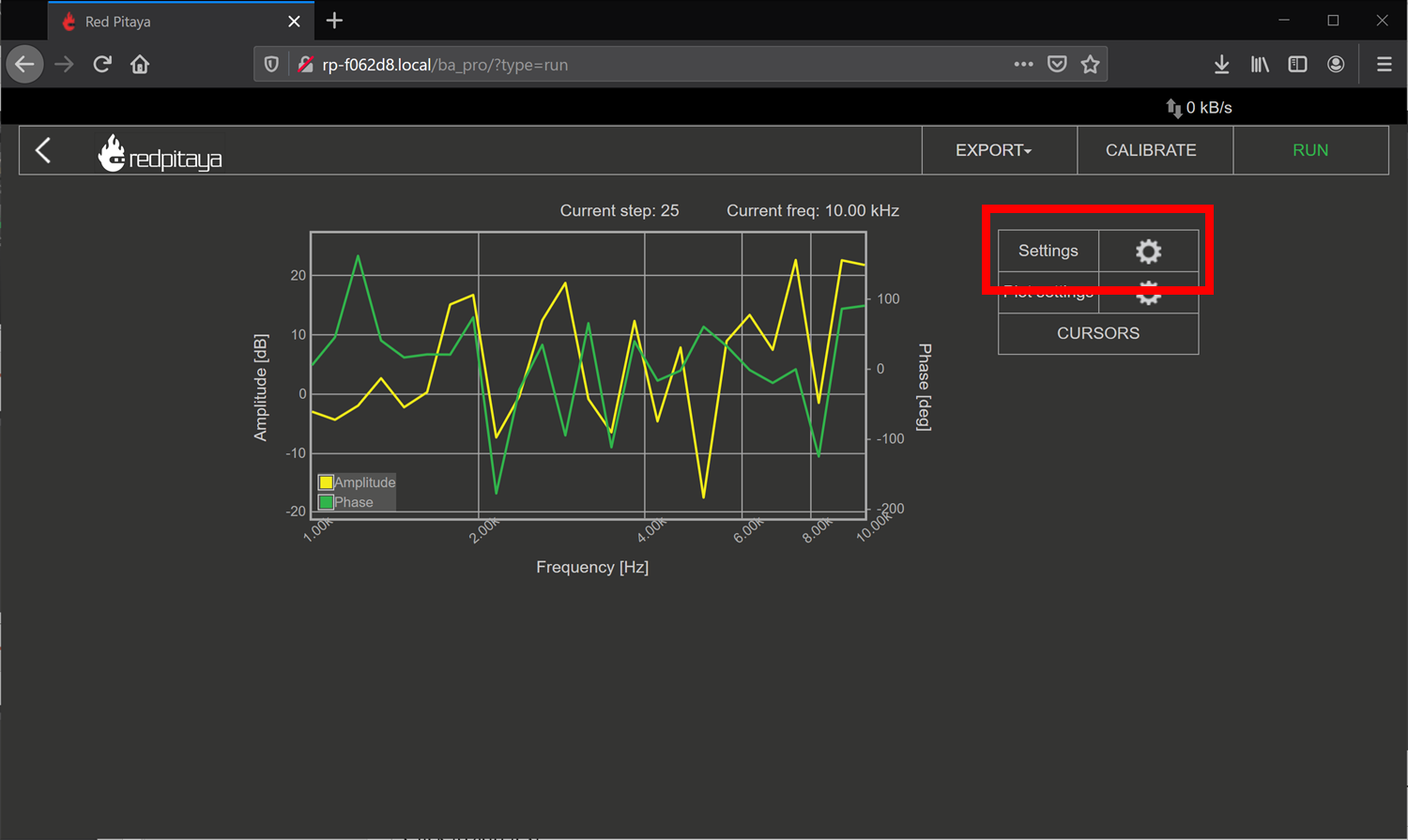
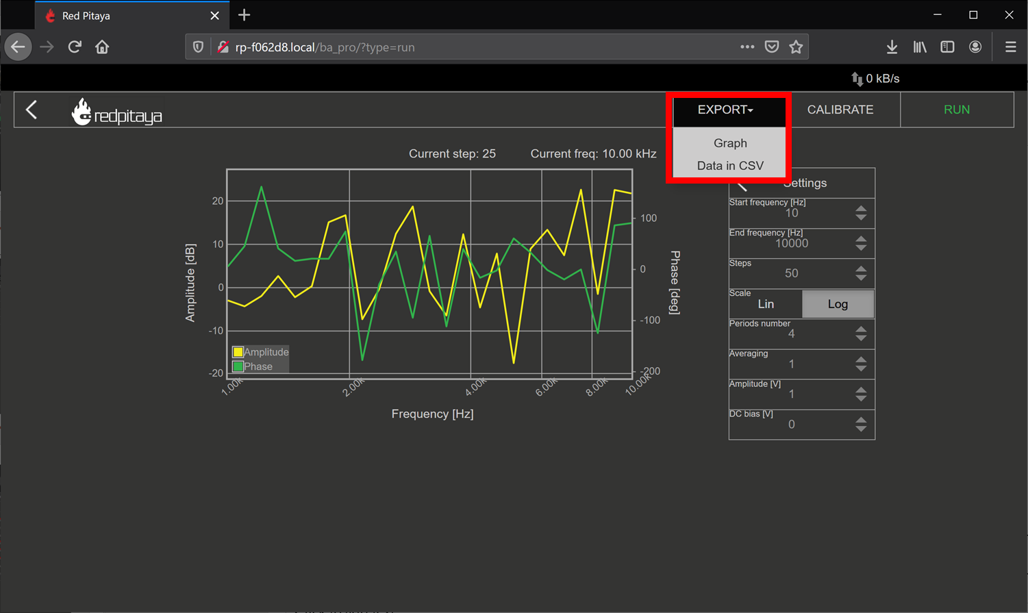
Click on the settings box to access the sweep settings
Configure the settings as shown below, we will find new sweep values as we go on, but these should be safe values to try
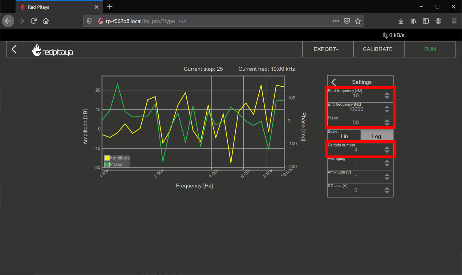
Click RUN – The sweep can take awhile to complete.
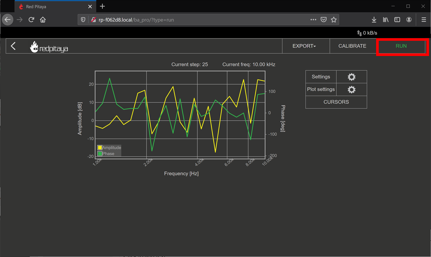
To export data: click the Export tab, and either select Graph for a PNG of the chart, or CSV for the raw CSV data of the plot.
Show the plot of the measurement below:
4.4.3.1.3. Comparison
Respond to the following questions:
Does the shape of the frequency response match your expectation from the analysis? Is there any point that stands out as odd?
Find the -3dB point in the circuit, and compare this value to the one you previously calculated.
4.4.3.2. Single stage RC circuit – 2
Build the Single stage RC circuit shown in Fig. 3, with \(R = 10k\Omega\),\(C = 0.47\mu F\).
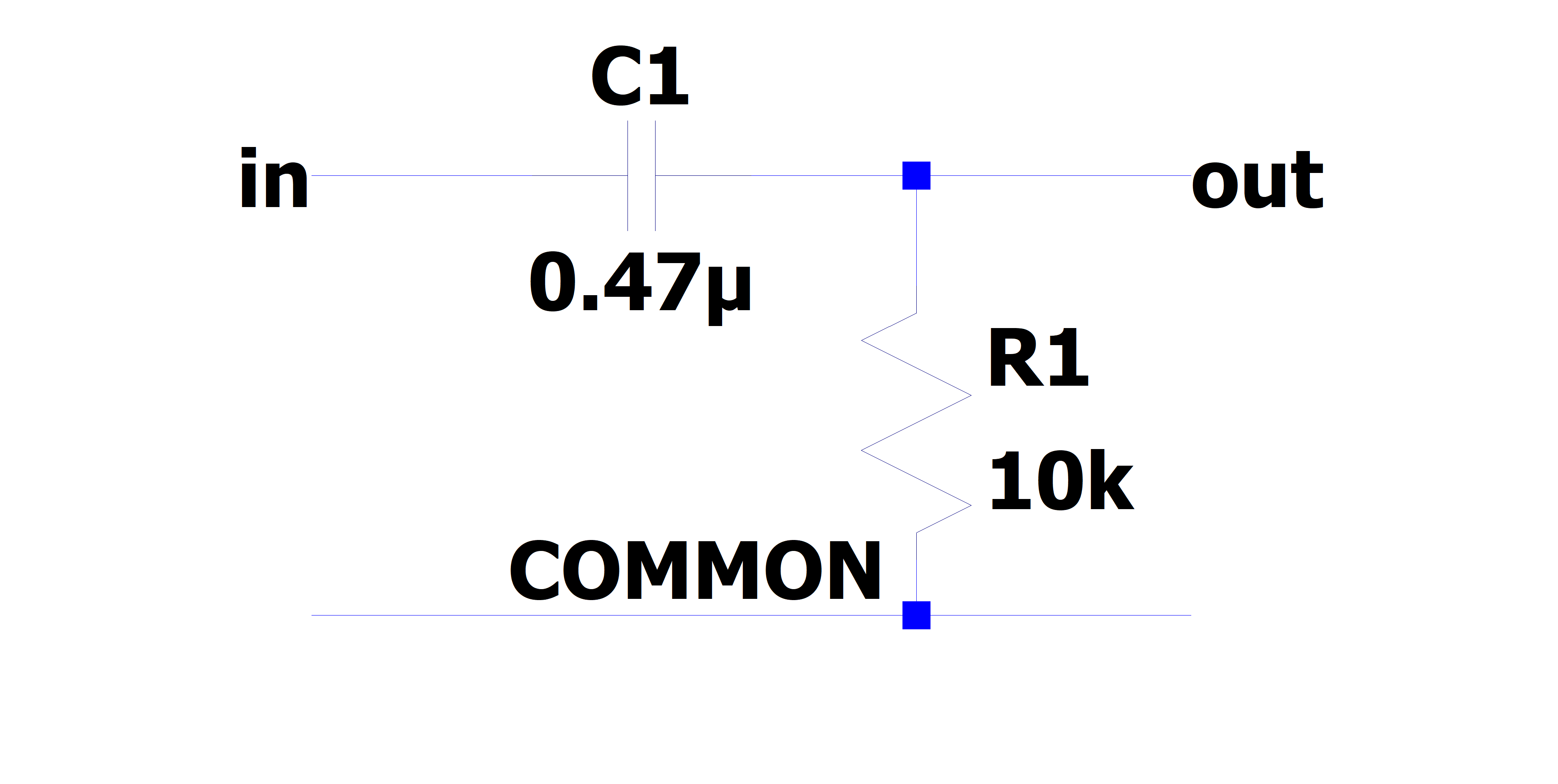
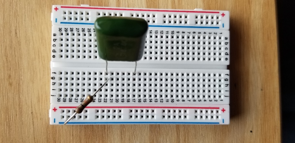
Fig. 3: (left) schematic of the single stage RC circuit, (right) implementation on breadboard
4.4.3.2.1. Analysis
The claimed transfer function of this circuit is
Where \(j = \sqrt{- 1}\) is the imaginary unit.
What is the magnitude of the transfer function?
What is the phase response of the circuit?
What class (low-pass, high-pass, band-pass, band-stop) of filter is this?
What is the -3dB frequency?
4.4.3.2.2. Measurement
Using the Red Pitaya’s Bode Analyzer tool, measure the frequency response (\(\left| T(f) \right|\)) as described in section 3.1.2.
Show the plot of the measurement below:
4.4.3.2.3. Comparison
Respond to the following questions:
Does the shape of the frequency response match your expectation from the analysis? Is there any point that stands out as odd?
Find the -3dB point in the circuit, and compare this value to the one you previously calculated.
4.4.3.3. Single stage RC circuit – Unknown parameter estimation
Build the Single stage RC circuit shown in Fig. 4, with the potentiometer and \(C = 4.7nF\). Use another resistor to provide electrical contact. Ensure that the potentiometer pins used are the two furthest pins, as this will be the total resistance of the device.
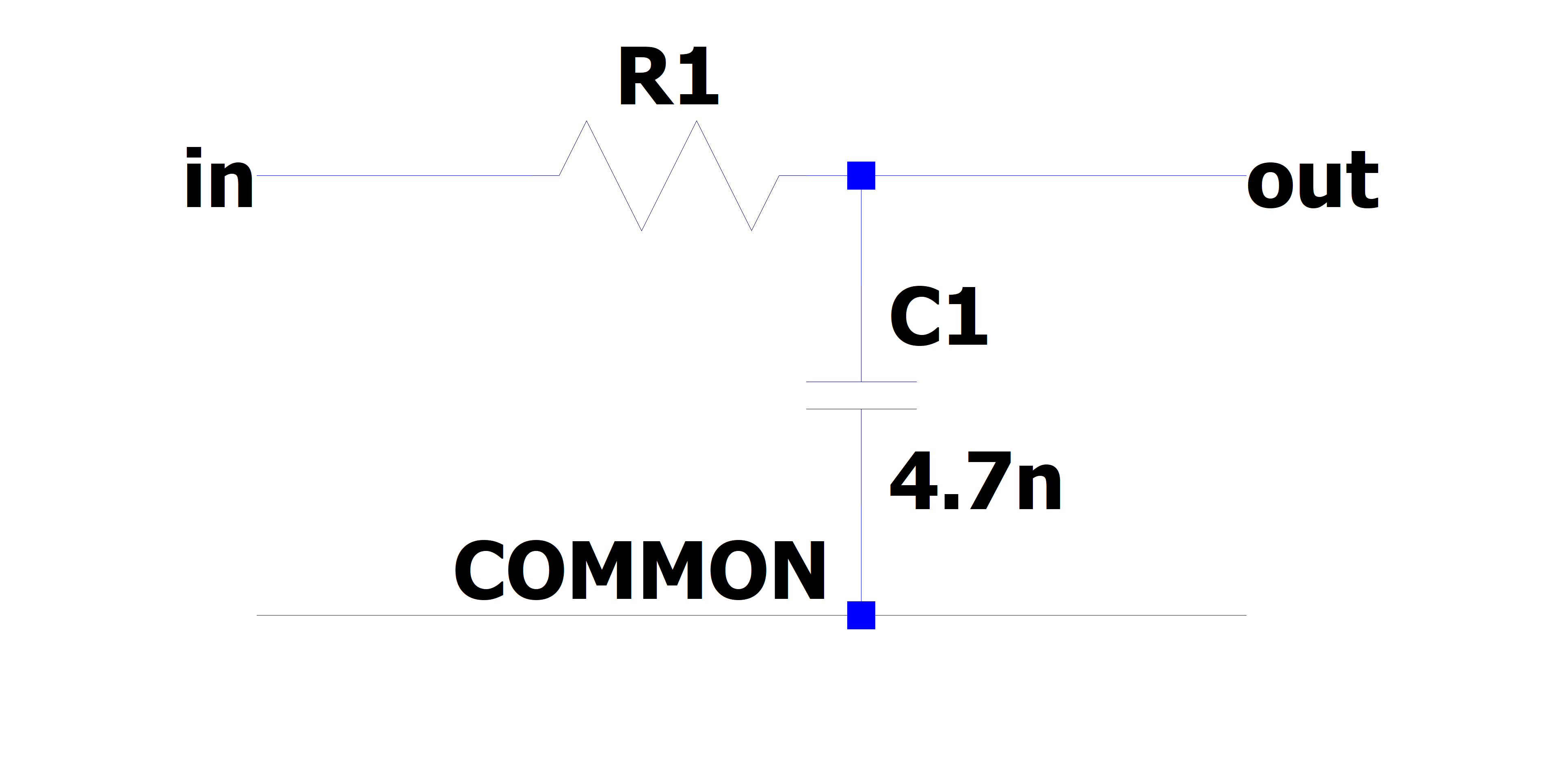
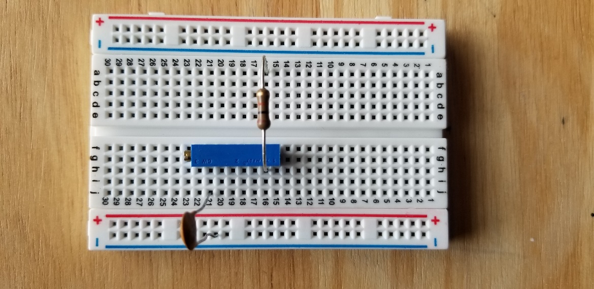
Fig. 4: (left) schematic of the single stage RC circuit, (right) implementation on breadboard
4.4.3.3.1. Analysis
The claimed transfer function of this circuit is the same as in 3.1 (reprinted here for courtesy)
Where \(j = \sqrt{- 1}\) is the imaginary unit. However now the value of \(R\) is unknown. Since we already know the expected behavior of the system, we can estimate the value of \(R\) by measuring the transfer function again.
Derive the expression for the -3dB frequency as a function of \(R\).
4.4.3.3.2. Measurement
Using the Red Pitaya’s Bode Analyzer tool, measure the frequency response (\(\left| T(f) \right|\)) as described in section 3.1.2. Pay special attention to include the cutoff frequency in the sweep.
Show the plot of the measurement below:
4.4.3.3.3. Comparison
Respond to the following questions:
Use the expression you derived to calculate the value of \(R\) from the measured value of \(f_{c}\).
To calculate the value of :math:R from the measured value of :math:f_c, we can rearrange the transfer function equation as follows: :math:T(f) = frac{1}{1 + j2pi fRC}. Solving for :math:R, we get :math:R = frac{1}{2pi f_cC}. Substitute the measured value of :math:f_c and the known value of :math:C to obtain the calculated value of :math:R.
The previous analysis all presumed we knew the value of \(f,C\) perfectly. In reality, the values of there are only approximately known.
If the capacitance value \(C\) can vary \(\pm 20\%\), what is the bounds on the error of the calculated value of \(R\)?
If the capacitance value varies by :math:pm 20%, the bounds on the error of the calculated value of :math:R can be determined by considering the sensitivity of :math:R with respect to :math:C. Using the formula for sensitivity, the upper bound of the error in :math:R can be calculated as :math:Delta R = left| frac{dR}{dC} right| cdot 0.2C, where :math:frac{dR}{dC} is the derivative of :math:R with respect to :math:C. Similarly, the lower bound can be obtained by considering the negative change (-20%) in capacitance.
If the frequency \(f\) value can vary \(\pm 0.1\%\), what is the bounds on the error of the calculated value of \(R\)?
If the frequency value varies by :math:pm 0.1%, the bounds on the error of the calculated value of :math:R can be determined by considering the sensitivity of :math:R with respect to :math:f. Using the formula for sensitivity, the upper bound of the error in :math:R can be calculated as :math:Delta R = left| frac{dR}{df} right| cdot 0.001f, where :math:frac{dR}{df} is the derivative of :math:R with respect to :math:f. Similarly, the lower bound can be obtained by considering the negative change (-0.1%) in frequency.
If the both \(C,f\) as above simultaneously, what is the total bounding on the error of the calculated value of \(R\)? (Hint: This should be a rectangular area)
If both :math:C and :math:f vary simultaneously, the total bounding on the error of the calculated value of :math:R can be obtained by combining the individual bounds calculated in parts (a) and (b). The total bounding will form a rectangular area defined by the maximum and minimum values of the error in :math:R due to the variations in :math:C and :math:f.
(Optional) In the same line of thought, assume that the values of \(C,f\) are described statistically by gaussian distributions with mean and variances provided below:
4.4.3.4. Cascading filters – Repeated stages
Build the RC circuit shown in below, with \(R_{1} = R_{2} = 10k\Omega\),\(\ C_{1} = C_{2} = 4.7nF\).
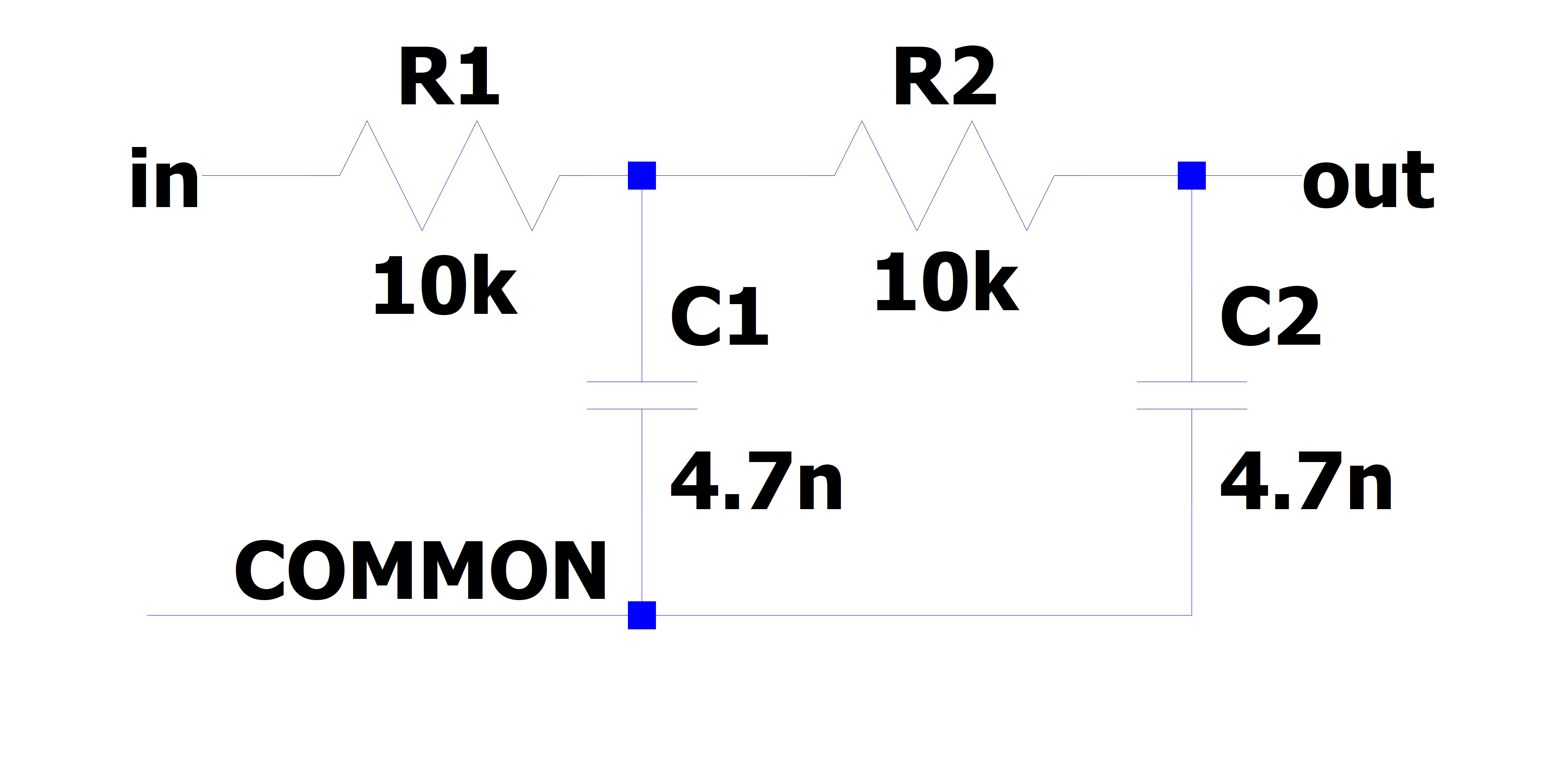
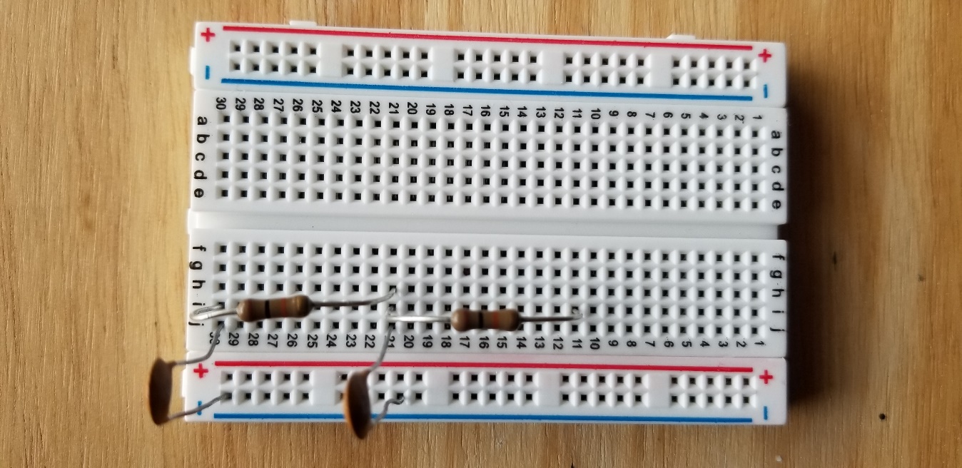
Fig. 5: (left) schematic of the single stage RC circuit, (right) implementation on breadboard
4.4.3.4.1. Analysis
The claimed transfer function of this circuit is
Where \(j = \sqrt{- 1}\) is the imaginary unit.
What is the magnitude of the transfer function?
What is the phase response of the circuit?
What class (low-pass, high-pass, band-pass, band-stop) of filter is this?
What is the -3dB frequency?
4.4.3.4.2. Measurement
Using the Red Pitaya’s Bode Analyzer tool, measure the frequency response (\(\left| T(f) \right|\)) as described in section 3.1.2.
Show the plot of the measurement below:
4.4.3.4.3. Comparison
Respond to the following questions:
Does the shape of the frequency response match your expectation from the analysis? Is there any point that stands out as odd?
Find the -3dB point in the circuit, and compare this value to the one you previously calculated.
This circuit can be viewed as two separate 1st order filters (see section 3.1) cascaded. What would the expected transfer function of such an arrangement look like? How different is this the expression you would expect from two ideal LTI systems?
4.4.3.5. Cascading filters – variable stages
Build the filter shown below, with \(R_{1}\) using the potentiometer as constant resistance. Once again, use the other 10K resistor as an electrical contact.
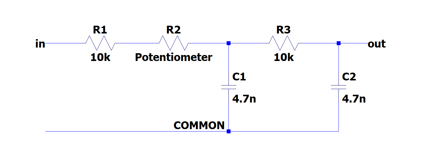
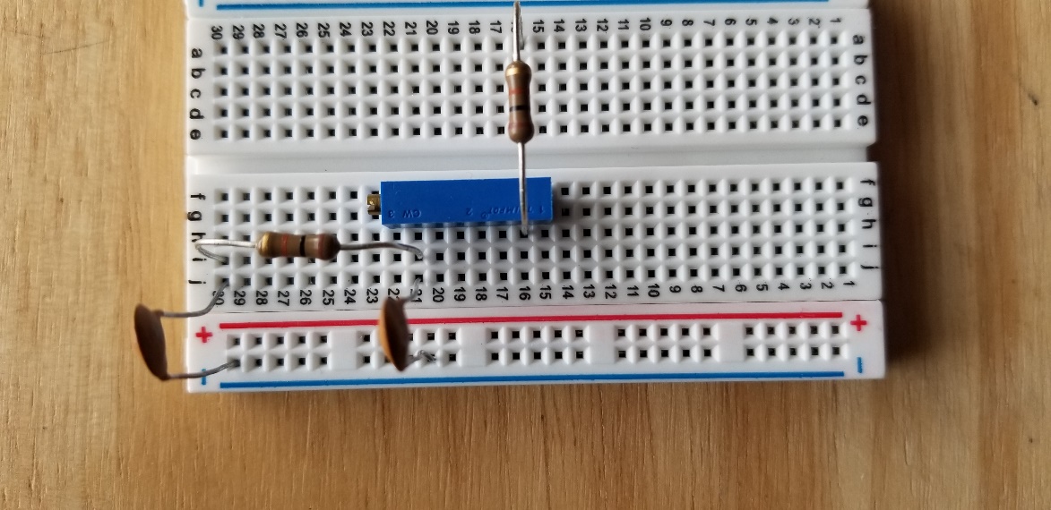
Fig. 6: (left) schematic of the single stage RC circuit, (right) implementation on breadboard
4.4.3.5.1. Analysis
The claimed transfer function of this circuit is
Where \(j = \sqrt{- 1}\) is the imaginary unit.
What is the magnitude of the transfer function?
What is the phase response of the circuit?
What class (low-pass, high-pass, band-pass, band-stop) of filter is this?
What is the -3dB frequency?
4.4.3.5.2. Measurement
Using the Red Pitaya’s Bode Analyzer tool, measure the frequency response (\(\left| T(f) \right|\)) as described in section 3.1.2.
Show the plot of the measurement below:
(Optional) Try sweeping from 10Hz to 1MHz. Is there anything strange that happens to the frequency response? Capture the frequency response, and describe what seems to happen to the transfer function.
4.4.3.5.3. Comparison
Respond to the following questions:
Does the shape of the frequency response match your expectation from the analysis? Is there any point that stands out as odd?
Find the -3dB point in the circuit, and compare this value to the one you previously calculated.
4.4.3.6. Questions and Answers
What is the magnitude of the transfer function?
The magnitude of the transfer function, denoted as \(\left| T(f) \right|\), represents the ratio of the output voltage \(V_{out}(f)\) to the input voltage \(V_{in}(f)\). In the given transfer function expression, the magnitude can be calculated as \(\left| T(f) \right| = \frac{1}{\sqrt{1 + (2\pi fRC)^2}}\).
What is the phase response of the circuit?
The phase response of the circuit, denoted as \(\phi(f)\), represents the phase shift between the input and output signals. In the given transfer function expression, the phase response can be calculated as \(\phi(f) = -\arctan(2\pi fRC)\).
What class (low-pass, high-pass, band-pass, band-stop) of filter is this?
The class of the filter can be determined by analyzing the transfer function. In this case, since the magnitude of the transfer function decreases with increasing frequency, it is a low-pass filter. A low-pass filter allows low-frequency signals to pass through while attenuating high-frequency signals.
What is the -3dB frequency?
The -3dB frequency, denoted as \(f_{c}\), corresponds to the frequency at which the magnitude of the transfer function is reduced to \(\frac{1}{\sqrt{2}}\) or approximately 0.707. Mathematically, it can be found by solving the equation \(\frac{1}{\sqrt{1 + (2\pi f_{c}RC)^2}} = \frac{1}{\sqrt{2}}\).
4.4.3.7. Conclusion
In conclusion, measuring the frequency response of a circuit is a valuable tool for evaluating its performance and validating theoretical models. By comparing the measured results with the expected behavior, we can identify any discrepancies and refine our understanding of the circuit’s characteristics. Additionally, accounting for uncertainties in component values enhances the accuracy of our analysis. Overall, frequency response measurements provide crucial insights for circuit design, optimization, and ensuring desired functionality in practical applications.