4.3. Modulation with the Red Pitaya

4.3.1. Introduction

Signal modulation plays a pivotal role in telecommunications, making it possible to transmit information across significant distances. To gain a practical understanding of modulation principles, this exercise utilizes the Red Pitaya, a versatile, open-source, software-defined radio (SDR) platform. The Red Pitaya enables us to generate and modify signals, facilitating the exploration of key concepts such as mixing, Amplitude Modulation (AM), and the impact of frequency normalization. This hands-on approach bridges the gap between theory and practice, allowing users to delve into the intricacies of signal modulation in a tangible way.

4.3.2. Mixing

The operation of mixing involves combining two signals together, usually through a multiplication operation. The result of multiplying two signals is a process that creates sum and difference frequencies from the original frequencies.

In the analysis of mixing, two sinusoids were used because sinusoids are the basis functions for Fourier Analysis, and any periodic signal can be represented as a combination of sinusoids (according to the Fourier Series). As such, it provides a straightforward way to visualize and analyze the principles of mixing and modulation.

To achieve this modulation, we can view the mathematical result of multiplying two periodic waveforms. For this analysis case, we will employ two sinusoids.

\[\begin{split}\begin{matrix} x_{1}(t) = A_{1}\cos\left( \omega_{1}t + \phi_{1} \right)x_{2}(t) = A_{2}\cos\left( \omega_{2}t + \phi_{2} \right)\ \#(1) \\ \end{matrix}\end{split}\]

Multiplying these two is made simple by invoking the well known trig identity:

\[\begin{split}\begin{matrix} \cos(x)\cos(y) = \frac{1}{2}\left\lbrack \cos(x - y) + cos(x + y) \right\rbrack\#(2) \\ \end{matrix}\end{split}\]

thus allowing:

\[\begin{split}\begin{matrix} x_{1}(t)x_{2}(t) = \frac{A_{1}A_{2}}{2}\left\lbrack \cos\left( \omega_{1}t + \phi_{1} - \left\lbrack \omega_{2}t + \phi_{2} \right\rbrack \right) + cos\left( \omega_{1}t + \phi_{1} + \left\lbrack \omega_{2}t + \phi_{2} \right\rbrack \right) \right\rbrack\ \#(3) \\ \end{matrix}\end{split}\]

This shows that:

We generate data at the sum and difference frequencies
Phases add directly
The amplitude/energy of the resulting data is shared from both waveforms

In most mixing applications, the results of a mixer are then filtered to only include either the sum or the difference frequency.

4.3.3. AM modulation

Amplitude modulation (AM) is a simple yet effective modulation scheme where the message signal (information to be sent) changes the amplitude of a faster “carrier” signal. The carrier signal is the base waveform that is modified to carry the information. It is typically a high-frequency sinusoid, chosen because it can easily propagate through space as a radio wave.

Amplitude modulation involves using a message signal (bandlimited to \(f_{m}\)) to modulate the amplitude of a faster “carrier” signal at \(f_{c}\). For simplicity, we will take the carrier to have no phase (this is justified by (3), where we can see that the mixed results simple add phase, and we can simply define \(\phi_{1} = 0\)), and give the modulated signal some phase \(\phi\).

\[\begin{split}\begin{matrix} \begin{matrix} x_{c}(t) = A_{c}\cos\left( \omega_{c}t \right) \\ x_{m}(t) = A_{m}\cos\left( \omega_{m}t + \phi \right) \\ \end{matrix}\ \#(4) \\ \end{matrix}\end{split}\]

4.3.3.1. Dual Side Band (DSB) Modulation

In Dual Side Band modulation, both the upper and lower sidebands are transmitted. This effectively doubles the bandwidth required for transmission. DSB modulation is relatively straightforward, but is not the most efficient in terms of bandwidth utilization.

Employing the simplest mixing, we simply multiple the carrier (denoted \(x_{c}(t)\)) by the message signal (denoted \(x_{m}(t)\)). This makes the resulting signal \(x_{DSB}(t)\)

\[\begin{split}\begin{matrix} x_{DSB}(t) = \ x_{c}(t)x_{m}(t) = \frac{1}{K}\frac{A_{c}A_{m}}{2}\left\lbrack \cos\left( \omega_{c}t - \left\lbrack \omega_{m}t + \phi \right\rbrack \right) + cos\left( \omega_{c}t + \left\lbrack \omega_{m}t + \phi \right\rbrack \right) \right\rbrack\ \#(5) \\ \end{matrix}\end{split}\]

This is what is known as Dual Side Band (DSB) or suppressed carrier modulation.

4.3.3.2. Amplitude Modulation

The traditional AM scheme includes a DC offset which allows the receiver to easily detect and remove the carrier signal and recover the original message. It is used because it is simple and the receiver circuitry is also simple. However, it is not power efficient as it needs to transmit the carrier along with the signal.

A more traditional AM modulation method for AM modulation employs a slightly modified version of DSB modulation. This time, the modulating signal is 1) scaled by the carrier amplitude, and 2) given a DC offset. This makes the new modulation function \(m(t)\) take the form

\[\begin{split}\begin{matrix} m(t) = 1 + \frac{x_{m}(t)}{A_{c}}\ \#(6) \\ \end{matrix}\end{split}\]

This makes the modulated signal simply \(x_{AM}(t) = x_{c}(t)m(t)\). This can be shown with some more clever trig identities to take the form

\[\begin{split}\begin{matrix} x_{AM}(t) = A_{c}\cos(2\pi f) + \frac{A_{c}}{2}\left\lbrack \cos\left( \omega_{c}t - \left\lbrack \omega_{m}t + \phi \right\rbrack \right) + cos\left( \omega_{c}t + \left\lbrack \omega_{m}t + \phi \right\rbrack \right) \right\rbrack\ \#(7) \\ \end{matrix}\end{split}\]

4.3.3.3. Sidenote: Modulation Index

The modulation index is a key parameter of any AM signal. It defines the extent of the variation in a carrier signal according to the information being sent. A high modulation index will cause a large amount of variation in the carrier signal, making it more susceptible to distortion or noise, while a low modulation index will lead to a lower signal quality.

Since there are now two terms, a carrier and the encoded message signal, we can consider the case of analyzing the peak of the message signal compared to the peak of the carrier. This ratio is known as the modulation index \(\mu\), and describes the modulation “strength” of the message onto the carrier.

\[\begin{split}\begin{matrix} \mu = \frac{\left| m(t) \right|}{A_{c}}\ \#(8) \\ \end{matrix}\end{split}\]

Full strengths modulation corresponds to a 100% index, and means that potential peaks of the carrier can be suppressed into a null. This parameter is not so important for this lab, but will be of interest to the analysis of communication systems in a future course.

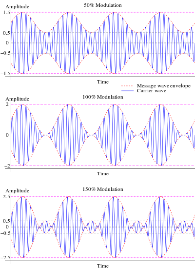
Figure : Modulation Index visualized. Credit: Wikipedia Modulation

4.3.3.4. Normalized Frequency

Frequency normalization is often employed in discrete systems to facilitate comparison between systems of different sizes or specifications. Normalized frequency is simply the frequency represented in terms of the Nyquist frequency or the sampling rate, thereby abstracting away the actual values and instead focusing on the underlying behavior of the system.

After the act of sampling, it becomes convenient to rescale (normalize) frequency w.r.t. the sampling frequency. This is done by the relation

\[\begin{split}\begin{matrix} \widehat{\omega} = \omega T_{s} = \frac{2\pi f}{f_{s}}\ \#(8) \\ \end{matrix}\end{split}\]

Where \(\omega = 2\pi f\) and \(T_{s} = 1/f_{s}\) is the sampling time. This representation is oftentimes used in discrete time systems as it allows for the consideration of systems in reference to the total bandwidth of the discrete system.

4.3.4. Tasks/Questions

4.3.4.1. Theory

Why in the analysis of mixing, were two sinusoids used? (Hint, sinusoids are what for the space of periodic functions?)

Two sinusoids were used because sinusoids form the basis of the space of periodic functions (Fourier series). In other words, any periodic function can be represented as a sum of sinusoids of various frequencies, amplitudes, and phases.
Why is the carrier being a sinusoid preferrable from a transmission perspective?

A sinusoid is preferable as a carrier signal because it is easy to generate, mathematically tractable, and well-suited for transmission over a medium (such as air for radio). Its constant amplitude makes it less prone to distortion as it propagates.
In both described AM schemes (DSB, AM w/modulation index), is there a way to reduce the total bandwidth of the system anymore? (Hint, do you need both sides of a spectrum to retrieve a signal if you know the signal is real valued?)

In DSB and traditional AM, there’s redundancy because the information is contained in both the upper and lower sidebands. If the signal is real-valued (as is often the case), you can use single-sideband (SSB) modulation, which cuts the bandwidth requirement in half.*

It was stated in the theory, that for AM, usually \(f_{c} > 10x\ f_{m}\). Why would this be true, and why would one want \(f_{c}\) to be even larger. For example, FM radio operates on a carrier of \(\approx 88 - 108MHz\), but the bandwidth of audio signals is only \(20kHz\) (as was demonstrated last lab).

:math:f_{c} > 10xf_{m} is often chosen to ensure the message signal doesn’t interfere with the carrier signal, to simplify the process of demodulation, and to adhere to regulations that prevent signals from occupying too much bandwidth. Also, a higher :math:f_{c} allows for better propagation of the signal.
Why is the carrier generally a very powerful signal in real systems? (Hint: how far are you from the radio tower when you listen to the radio? As all signals travel, they will spread out unless coerced otherwise)

The carrier signal is powerful in real systems because as signals travel, they lose power due to various factors (like propagation loss). A stronger carrier signal ensures that the signal can be received at a greater distance from the transmitter.

4.3.5. Experiment

Set the frequency of the message signal to 0.1. Show a plot of the acquired waveform. What does a normalized frequency :math:widehat{omega} < frac{1}{2pi} mean, and why does it introduce odd behavior into the observed waveforms?

In this scenario, you would need to configure your Red Pitaya setup to generate a message signal with the specified frequency and observe the waveform. The acquired waveform can then be plotted using a suitable software tool (e.g., MATLAB or Python). A normalized frequency of :math:widehat{omega} < frac{1}{2pi} would suggest that the frequency of the signal is less than half the sampling frequency. This introduces odd behavior into the observed waveforms due to the phenomenon known as “aliasing,” where the signal is undersampled, causing it to appear as a lower frequency signal.

What happens when the message signal frequency is the same size or greater than the carrier frequency?

When the message signal frequency is the same size or greater than the carrier frequency, there could be issues with effective modulation. The carrier signal, as the name suggests, is supposed to “carry” the message signal, and it is typically of higher frequency. If the message frequency equals or surpasses the carrier frequency, the information might not be effectively encoded into the carrier signal, leading to poor reception or loss of data.

Use a message signal that is not a pure sinusoid (e.g. use anything that is a superposition of sinusoids), show the resulting spectrum, and comment as to the bandwidth of the modulated signal.

When a message signal that is not a pure sinusoid, e.g., a signal that is a superposition of sinusoids, is used, the resulting spectrum shows peaks at the frequencies of the individual sinusoids. The bandwidth of the modulated signal, in this case, will be broader. This is because the modulated signal now carries the information of multiple sinusoids, each with its own frequency, thus widening the total range of frequencies (bandwidth) in the signal.

Use a carrier signal that is not a pure sinusoid (e.g. use the square function), show the resulting spectrum, and comment as to the resulting signal strength in any one peak when compared to a pure sinusoidal carrier.

When a carrier signal is not a pure sinusoid, such as a square wave, the resulting spectrum of the modulated signal would contain additional harmonics due to the rich harmonic content of the square wave. The strength of the signal at any one peak could potentially be less than that of a pure sinusoidal carrier. This is because the energy of the square wave is distributed across several harmonics, while a pure sinusoidal carrier concentrates all its power at a single frequency.

Demonstrate aliasing with the modulated signal. This will involve you setting the message signal to have frequency content that passes the sampling frequency when modulated by the carrier. Show a plot of the aliased content in the time domain, and the frequency domain.

Aliasing with the modulated signal can be demonstrated by choosing a message signal with frequency content that, when modulated by the carrier, exceeds the sampling frequency. In such a case, the sampling theorem is violated and aliasing occurs. Aliasing is a form of distortion where higher frequency components get mapped onto lower frequencies. A plot of the time-domain signal will show this as distortions or anomalies in the signal, while in the frequency domain, you would see mirrored content about the Nyquist frequency. Remember, the exact appearance of aliasing will depend on the specific frequencies of your message and carrier signals, as well as your sampling frequency.

4.3.6. Conclusion

In conclusion, the Red Pitaya platform provides an effective, hands-on method for exploring signal modulation techniques, such as mixing and amplitude modulation. It allows users to directly observe the effects of varying signal frequencies and shapes, revealing the impacts of phenomena like aliasing. Despite some potential deviations from ideal scenarios due to hardware limitations or environmental noise, the Red Pitaya serves as a valuable learning tool for bridging theoretical principles with practical applications in signal processing and modulation.