4.6. Digital Filtering on the Red Pitaya
4.6.1. Introduction
Red Pitaya, an open-source tool combining numerous measurement and control instruments, is an ideal platform for exploring digital signal processing (DSP), specifically digital filtering. Digital filters manipulate signal characteristics, performing tasks like noise removal and signal smoothing.
4.6.2. Theory
4.6.2.1. Z-Domain LTI Systems
It’s important to remember that all discrete time LTI (Linear Time-Invariant) systems can be formulated in a canonical form:
Here, the coefficients of each term in the equation can be perceived as the coefficients in the corresponding difference equation:
4.6.2.2. Filter Design Basics
When designing a filter, the order plays a significant role in determining its performance characteristics. The order of a filter is often considered in terms of the filter’s ‘sharpness’ in transitioning from the passband to the stopband. A higher order filter results in a steeper roll-off, allowing for a sharper transition. However, this comes with the drawback of potentially introducing more phase distortion.
A simple first-order low-pass filter has the following transfer function in the s-domain:
where \(T\) is the time constant of the filter. The higher the order of the filter, the more complex this equation becomes.
4.6.2.3. Windowing in Digital Filters
In digital FIR filter design, windowing techniques involve the multiplication of an ideal impulse response with a window function. The selection of a window function impacts the trade-offs between side lobe level, transition width, and main lobe width.
A general formula for the FIR filter coefficients using windowing can be represented as:
where \(h_d[n]\) is the impulse response of an ideal filter, \(w[n]\) is the window function, and \(n\) ranges from 0 to N-1.
4.6.2.4. The Power of IIR Filters
Unlike FIR filters, Infinite Impulse Response (IIR) filters have both poles and zeros, meaning their impulse response can theoretically continue indefinitely. A basic first-order IIR filter has a transfer function given by:
where \(b_0\) and \(b_1\) are feedforward coefficients and \(a_1\) is a feedback coefficient. Higher order IIR filters have more complex transfer functions, with additional ‘b’ and ‘a’ coefficients.
4.6.2.5. A Glimpse into Digital Signal Processing
The Nyquist-Shannon sampling theorem states that a continuous time signal can be properly sampled, only if it does not contain frequency components above half of the sampling rate. If the condition is not satisfied, aliasing occurs. In mathematical terms, for a signal with a maximum frequency component of \(B\) Hz, the sampling frequency \(f_s\) should be:
The Discrete Fourier Transform (DFT) transforms a finite sequence of equally-spaced samples of a function into an equivalent sequence of samples in the frequency domain. Its general equation can be written as:
The convolution operation, denoted by ‘*’, is used to find the output \(y[n]\) of an LTI system, given an input \(x[n]\) and an impulse response \(h[n]\):
The Z-transform maps a sequence of numbers in the time domain into a sequence in the complex frequency domain. It is defined by:
where \(x[n]\) is the discrete-time input signal and \(X (z)\) is the Z-transform of \(x[n]\). This tool proves to be instrumental in the analysis and design of digital filters.
Digital filters are designed to perform various operations on signals such as amplification, attenuation, or specific frequency content modification. The filter’s functionality can be described by a difference equation. For instance, a generic form of a first-order (one-pole) discrete-time system is described by:
where \(y[n]\) is the output, \(x[n]\) is the input, \(a_1\) and \(b_0\) are the filter coefficients. This equation exemplifies how the output signal at a specific time ‘n’ depends on the previous output and the current input.
With the digital representation of signals and systems, we can leverage computational resources to perform complex processing tasks, analyze the behavior of systems, and design intricate signal processing architectures. The theory behind digital signal processing sets the foundation for the tasks and analysis that follow in this text.
4.6.3. Hands on experiment
4.6.3.1. Hardware configuration
This configuration will require an additional piece of equipment, a
second red pitaya. One red pitaya will be used as in the
oscilloscope/signal generator or the spectrum analyzer modes, while the
other will be used in the LTI DSP workbench. Connect the red pitayas
such that the IN1 of the LTI DSP device is connected to OUT1 of the
generator. You can also use a T-joint to connect the OUT1 of the
generator board to IN1 of itself to see the response of the circuits
more clearly and to measure the Frequency response with the Bode
analyzer. 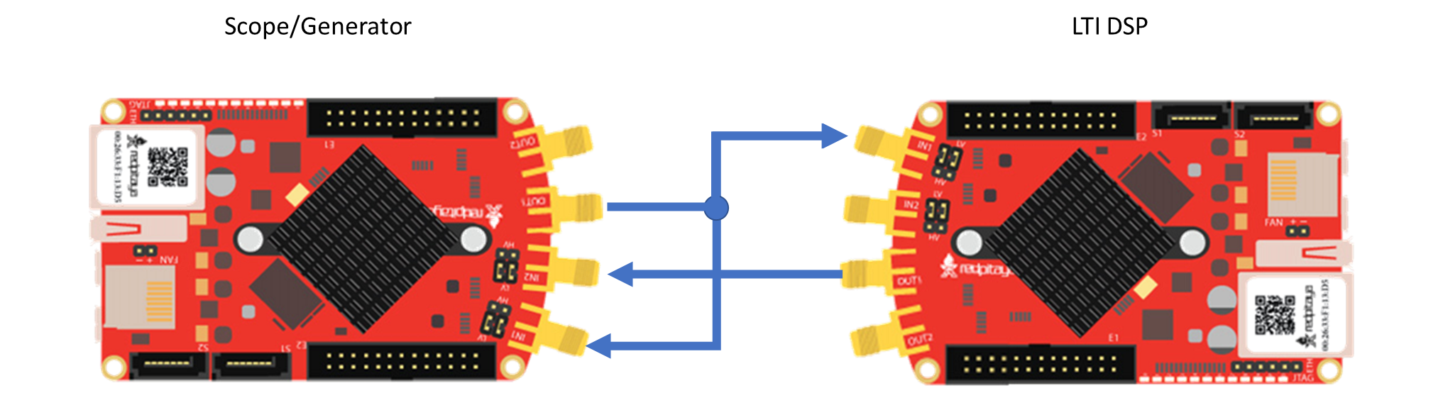
4.6.3.2. All-Pass Filter – Delay Element
Enter the following transfer function into the LTI workbench:
This is accomplished by setting \(b_{0} = 1\). This kind of filter is called an all pass filter, due to its input/output relation of simply passing the output. Note that this is a special class of all-pass filter, namely a delay filter. This kind of filter purely provides a delayed version of the input as it’s output.
4.6.3.2.1. Measurement
Note down the Bode plot from the LTI workbench for both gain and phase(Note for some filters, you may want to do this over two screenshots, as the magnitude and phase are plotted on a common axis, even if one is in dB and the other is in degrees), and describe what happens as the frequency of the input signals are increased or decreased. (Hint: refer to the frequency response from the LTI workbench)
Since this is an all-pass filter, the Bode plot should ideally show a flat magnitude response indicating a gain of 1 (or 0 dB) at all frequencies. The phase response would ideally be linear, indicating that each frequency component of the signal is delayed by the same amount. As you increase or decrease the frequency, the phase delay should correspondingly increase or decrease.
Show the resulting waveform in the Red Pitaya/Spectrum Analyzer scope object for
A sine wave of 1kHz is applied
A square wave of 1kHz is applied
A triangle wave of 1kHz is applied
4.6.3.2.2. Analysis
Is this also an all pass filter? Why or why not?
The function H(z) = z^(-k)/1 is indeed an all-pass filter. This filter introduces a delay of ‘k’ samples to the input signal but does not change the magnitude of any frequency component, hence qualifying as an all-pass filter.
If I wanted to attenuate the incoming by 50% (multiply by 0.5) what would the general all-pass filter function be?
To attenuate the incoming signal by 50%, the transfer function would be: :math:`H(z) = 0.5*z^(-k)/1`. This introduces a delay while halving the magnitude of the input signal.
Write out the difference equation for a general all pass filter.
The difference equation for a general all-pass filter would be:
4.6.3.3. Moving average filter
An \(n\)-tap moving average filter has the form:
This is accomplished by setting \(b_{k} = 1/N\\). This kind of filter is called a moving average or boxcar filter, due to its nature of taking a local average of \(n\) samples at every sample point. Oftentimes the size of \(N\) is known as the window size.
4.6.3.3.1. Measurement
Note down the Bode plot from the LTI workbench for both gain and phase for the provided value of \(N\), describing what happens as the frequency of the input signals are increased or decreased.
\(N = 3\)
\(N = 5\)
\(N = 6\)
What are the trends as \(N\) gets larger?
The Bode plot for a moving average filter will show that as the frequency of the input signal increases, the gain decreases. This is a characteristic of a low-pass filter. As N increases, the cut-off frequency of the filter decreases, and the filter becomes more selective.
Show the resulting waveform in the Red Pitaya/Spectrum Analyzer scope object for:
A sine wave of 1kHz is applied
A square wave of 1kHz is applied
A triangle wave of 1kHz is applied
4.6.3.3.2. Analysis
What class of filter does this look like? (high-pass, low-pass, band-pass, band-stop)
This filter is a low-pass filter.
What does the window size say about the filter’s performance?
The window size, N, determines the filter’s cut-off frequency and its selectivity. Larger N means lower cut-off frequency and higher selectivity.
Write out the difference equation of this filter.
The difference equation of this filter is:
4.6.3.4. Low pass filter
Enter the following transfer function into the LTI workbench:
4.6.3.4.1. Measurement
Note down the Bode plot from the LTI workbench for both gain and phase. (Note for some filters, you may want to do this over two screenshots, as the magnitude and phase are plotted on a common axis, even if one is in dB and the other is in degrees)
Show the resulting waveform in the Red Pitaya/Spectrum Analyzer scope object for:
A sine wave of 1kHz is applied
A square wave of 1kHz is applied
A triangle wave of 1kHz is applied
Describe what happens as the frequency of the input signals are increased or decreased.
For a low-pass filter, as the frequency increases, the gain decreases. This effect is more prominent after the cut-off frequency.
4.6.3.4.2. Analysis
Write out the difference equation of this filter.
In the previous lab, we showcased that low-pass filters can be used to approximate integral operations. At what frequency does this filter do a passable job of implementing this operation?
This filter does a passable job of implementing integral operations at low frequencies, usually below its cut-off frequency.
4.6.3.5. 1st difference filter
Enter the following transfer function into the LTI workbench:
This is accomplished by setting \(b_{0} = 0.5,\ b_{1} = - 0.5\).
4.6.3.5.1. Measurement
Note down the Bode plot from the LTI workbench for both gain and phase, and describe what happens as the frequency of the input signals are increased or decreased.
Show the resulting waveform in the Red Pitaya/Spectrum Analyzer scope object for:
A sine wave of 1kHz is applied
A square wave of 1kHz is applied
A triangle wave of 1kHz is applied
This filter should amplify the high frequencies while attenuating the low frequencies.
4.6.3.5.2. Analysis
What does removing the common factor of \(1/2\) do to the filter? Why do you think the factor of \(1/2\) was included?
Removing the 1/2 factor would double the gain of the filter. The factor of 1/2 was included to normalize the filter response.
Write out the difference equation of this filter.
In the previous lab, we showcased that high-pass filters can be used to approximate derivative operations. At what frequency does this filter do a passable job of implementing this operation?
This filter does a passable job of implementing derivative operations at high frequencies.
4.6.3.6. Feedback
Enter the following transfer function into the LTI workbench:
4.6.3.6.1. Measurement
Note down the Bode plot from the LTI workbench for both gain and phase. (Note for some filters, you may want to do this over two screenshots, as the magnitude and phase are plotted on a common axis, even if one is in dB and the other is in degrees)
Show the resulting waveform in the Red Pitaya/Spectrum Analyzer scope object for
A sine wave of 1kHz is applied
A square wave of 1kHz is applied
A triangle wave of 1kHz is applied
Describe what happens as the frequency of the input signals are increased or decreased.
The frequency response of this feedback filter would depend on the specific value of the feedback coefficient (0.93 in this case). The gain and phase response should be noted accordingly.
4.6.3.6.2. Analysis
Write out the difference equation of this filter.
[STRIKEOUT:In the previous lab, we showcased that low-pass filters can be used to approximate integral operations. At what frequency does this filter do a passable job of implementing this operation?]
4.6.4. Conclusion
In this series of experiments, we’ve explored different types of digital filters using the Red Pitaya and the LTI DSP workbench. We’ve studied an all-pass filter that passes all frequency components without alteration, a moving average filter acting as a low-pass filter, a dedicated low-pass filter, a first-difference high-pass filter, and a feedback filter.The study included a theoretical analysis of their transfer functions, prediction of their behavior based on Bode plots, and hypotheses about how these filters would alter the waveforms of input signals. We also examined the difference equations of these filters, which provide a time-domain representation of their operation.In conclusion, this exercise provides a solid basis for understanding how different types of digital filters function and how to implement and analyze them using real-world tools and equipment.